Ekonomika ISSN 1392-1258 eISSN 2424-6166

2024, vol. 103(1), pp. 127–144 DOI: https://doi.org/10.15388/Ekon.2024.103.1.8

What Is the Level of Savings Needed for High-Technology Export Led Growth?

Ebru Gül Yilmaz
İstanbul Gelişim University, Faculty of Economics, Administrative and Social Sciences,
Department of International Trade and Finance Department Avcılar İstanbul/TURKEY
Email: egyilmaz@gelisim.edu.tr
ORCID: https://orcid.org/0000-0002-3610-4982

Abstract. High-tech export-led growth is an important determinant in terms of having a milestone feature for the level of development of countries. Although the restrictions arise from recent literature, it is obvious that countries, like Korea with 35.7% the high-technology product export ratio and China with 31.3%, that have set a strategy on the high-technology export-led growth could have managed to achieve what they aimed to have. It is obvious that to make any investment in high-technology products, a certain level of savings should be achieved. The purpose of this paper is to determine the savings level that is necessary for achieving a high-technology export level for economic growth. The motivation arises from the willingness to shed light on policymakers on their way to achieve the high-technology export-led growth. Sixteen countries with high-technology product export levels higher than the World’s average are chosen in order to test the HXT export-led growth strategy at the initial stage. The period of 2007–2020 has been chosen due to the availability of the data. After achieving the result that there is a bidirectional casualty relationship between HTX and economic growth, by using the threshold regression model it is concluded that after achieving the savings level of 38.73%, countries can create an increase in their HTX level. And this is a very important output for policymakers for setting their strategies for the high-technology export-led growth. Hence the main aim of the policymakers is to increase welfare level of citizens, they should aim to reach 38.73% in order to achieve the high-technology export-led growth. After reaching this savings level they will have a chance to make investments for producing high-technology products by routing their savings to research and development and getting patents. In this way, they will have a chance to increase the welfare levels with the HTX-led growth strategy.
Keywords: High-technology export-led growth, saving level, Dimutrescue and Hurlin Casualty, Threshold Regression, Economic Development

______

Received: 19/04/2023. Revised: 09/10/2023. Accepted: 20/12/2023
Copyright © 2024 Ebru Gül Yilmaz. Published by Vilnius University Press
This is an Open Access article distributed under the terms of the Creative Commons Attribution License, which permits unrestricted use, distribution, and reproduction in any medium, provided the original author and source are credited.

1. Introduction

GDP growth has been one of the most important success indicators of governments for years and high-technology product exports are taken as a triggering factor for the growth of economies with the acceleration in technological improvements, especially in the last decades.

Welfare is an element that cannot be achieved by economic growth alone. It is essential to ensure development to increase welfare. After achieving a certain technological infrastructure, producing high-technology products and as a second step exporting the HTX products may be accepted as a criterion for economic development under recent global conditions.

This paper explores whether high-technology product export level causes any increase in economic growth or not as a first step, after the conclusion of this area, it defines the definite saving levels of countries in which they can achieve a satisfactory HTX export level. And it is distinct from the research in the literature by extending the HXT export and growth relationship to a crucial point which is defining the certain saving level at which countries can achieve a satisfactory HTX level.

Essentially, the starting point of this article is examining a growth model based on high-tech product exports. And the motivation is to define a certain saving level for achieving a satisfactory HTX level.

2. Theoretical Background

To explain in detail to the reader, the logical sequence that leads to the purpose of the article, technology as an indicator of development and ‘development and foreign trade’ will be taken into the theoretical background of the paper.

2.1. Economic Development and Technology

Technology itself has been taken as an external factor (Solow–Swan) for economic growth and later on is accepted as an internal factor (Romer and Lucas).

Total Factor Productivity, which was first mentioned by Robert M. Solow at 1957 and was explained in his research named ‘Technical Change and Aggregate Production Function.’ He defined the special form of neutral technical change which means marginal rates of substitution are untouched but there is a decrease or increase in outputs (Solow, 1957)

2.2. Economic Development and Saving

Savings are defined as the part of the income that is not consumed and is the difference between income and expenses. According to classical economic theory, saving is a function of interest rate: there is a direct relationship between the amount that individuals save at a given real income level and the real interest rate. Accordingly, the increase in real interest rates positively affects the saving tendency; the decrease in real interest rates affects the propensity to save negatively. According to Keynesian theory, saving is a function of income. Keynes has made a differentiation between full employment and underemployment conditions. The increase in consumption in an economy that has reached the full employment level causes the production factors used in investment goods to shift to consumption goods, and thus the increase in consumption causes a decrease in investments. Whereby if the economy is at underemployment equilibrium increase in consumption causes an increase in investments.

Individuals consume some part of their income, and they save the rest. Determining the level of saving when savings are equal to investments, i.e. I=S, means a closed economy. It will gain determining how much investment can be made becomes more important for economic development.

In addition to increasing the capital endowment of the national economy, the savings impact economic growth and development positively by providing opportunities for making investments in research and development and technology which lead to an increase in efficiency.

The average for the last two decades for the saving level of all countries in the world is 26.31% and the high-technology export level of the world for the same period is 19.99% (Figure 1).

Resources that can be used to realize technological investments in an economy can be divided into savings, bank loans and borrowings from organizations such as IFC and the World Bank, and foreign direct investments. For the last two decades, after facing with global crisis due to oil prices, the 2008 Mortgage Crisis, and high-level interest rates there occurred an international debt crisis. And most countries changed their strategies to reduce foreign debt and increase domestic savings.

Countries that set their strategies on producing and exporting high-technology products have managed a crucial acceleration in their GDP per capita levels such as Korea and China. In order to support the statement, some figures will be given on patent applications in China that have increased by 5399% in the years between 2000 and 2018. With this acceleration, the share of China in the World in terms of patent numbers is increased from 3% to 61%. Parallel to this, the GDP per capita of the country also has increased from 959 USD to 9,771 USD within the same time span with an increase of 919% (Yılmaz, 2020).

Technological backwardness stands out as a common feature of underdevelopment. The main reason for poverty, which can be considered in common, is that developing countries do not have sufficient capital accumulation and, accordingly, they cannot make progress in their technology level due to their inability to allocate sufficient resources for research and development activities.

8_1_pav.pdf

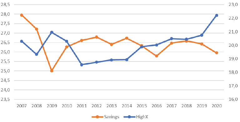
Figure 1: Worldwide Saving/GDP and HTX/Total Export Trend

Resource: World Bank (2022)

2.3. Economic Development and Foreign Trade

Theorems on foreign trade exhibit that foreign trade supports the development of countries by triggering competition and leading specialization in the sectors in which production factors are abundant, thus increasing productivity by leading to technology transfer. And by combining all theoretical backgrounds, savings which lead to an increase in technology levels of countries, and by producing and exporting high-technology products, achieving economic growth and development targets is the main underlying idea of this paper. Moreover, for the countries like China, Korea, Japan, Malaysia, Singapore, Norway, United Kingdom with high-level of HTX exports, it is seen that these countries also have high GDP per capita levels or the acceleration of their GDP per capita is parallel with their increase in HXT export levels. With all these facts the problem statement of the paper has been set as: there are some countries that managed to achieve high-technology-led growth and they are developing very fast whereby some others can’t. Can achieving a certain level of savings be an answer to this difference? If savings can provide an economic development via the HTX-led growth what is the specific level of the savings needed to achieve such a fast development? The hypothesis of the paper is as follows: in order to achieve the economic growth and development based on a high-technology export-led growth strategy, a certain level of savings is needed. Two-stage analysis is designed; at the initial stage the casualty relationship between HTX and economic growth will be analyzed by using the Dimutrescue–Hurlin test and after, proving the high-tech export-led growth hypothesis, threshold regression will be imposed to specify the saving level needed for the high-tech export-led growth. The only limitation can that be accepted is the difficulty in finding long-term data for the high-technology export. When it comes to contribution to the literature of this paper, it is proud to be the first research paper that exhibits the savings level needed for the HTX-led growth.

3. Literature

Research specific on the relationship between savings levels and high-tech exports could not be found in the literature, so a literature review was conducted on the determinants of high-tech product exports, the relationship between savings and economic growth, savings and investment and the relationship between economic growth and high-technology exports.

Aghion, Comin, Howitt, and Tecu (2016) have done research to get the answer to the question: ‘Can a country achieve a faster growth performance by increasing savings?’ They discuss this by handling poor and rich countries separately and conclude that the answer of the question is ‘yes’ for just poor countries, not for the rich ones.

Seyoum (2004) did research on 55 countries including both developing and developed countries and concluded that high-technology export is a function of inward foreign direct investment, technological infrastructure, and local demand conditions.

Braunerhjelm and Thulin (2008) tested the impact of research and development expenditure and country size on high-tech exports by working in 19 OECD countries for the years 1981–1999. They reported that country size does not have any impact on HTX but R&D expenses have a statistically significant impact on HTX.

Tebaldi (2011) defined FDI (foreign direct investments), human capital, openness, savings, gross capital formation, and macroeconomic volatility as candidate determinants of high-technology exports. By using panel data analysis, it was concluded that savings and gross capital formation have no effect on HTE (high-technology exports), on the other hand, FDI, human capital, and openness are the key indicators of HTE.

Gokmen and Turen (2013) have concluded that economic freedom level, human development level, and FDI, and high-technology exports have a bidirectional casualty relationship by imposing the Granger casualty test for 15 EU countries with the time span of 1995–2010.

Telatar et al. (2016) have concluded that there is a one-way casualty relationship between high-technology product exports and economic growth in Turkey from 1996 to 2015.

Ekananda & Parlinggoman (2017) have analyzed the effects of foreign direct investments, high-technology exports and non-high-technology exports on GDP for 50 countries from the time span of 1992–2014 and reported that both high-tech and non-high-tech exports have significant and positive effects on GDP but high-tech exports have a stronger impact.

Kabaklı, Duran and Üçler (2017) defined FDI, gross capital formation, patent application of residents and growth rate as candidates for determinants of high-technology product export. They imposed the Westerlund Cointegration test and the pooled mean group estimator for OECD countries for the time span of 1989–2015. They concluded that FDI and patent applications positively and significantly impact HTX.

Usman (2017) has analyzed the effects of high-tech exports on growth for the years 1995–2014 by imposing the ordinary least square method and concluded that high-tech export has an important role in long-run growth.

Demir (2018) has worked in 34 countries to determine the effects of high-technology and middle-technology on economic growth by using dynamic panel data analysis. He has concluded that both high- and middle-technology product exports have positive impact on economic growth

Satrovic (2018) has noted a bidirectional relationship between economic growth and HTX by applying the Granger causality test for 70 countries between 1995 and 2015.

Joshi et al. (2019) revealed that savings has a negative impact on economic growth in Nepal.

Şahin (2019) imposed the Granger causality method, and the findings have revealed that high-technology export has a positive impact on the economic growth in Turkey with the time span of 1989–2017.

Singh (2019) imposed FMOLS and FIML estimates in order to test the relationship between savings and investments for 24 OECD countries and concluded that there is a cointegration relationship between savings and investments.

Gunes, Gurel, Karadam, and Akın (2020) found out that FDI (Foreign Direct Investments), trade openness, schooling, and per capita income are the determinants of HTE-high technology exports by employing the ARDL methodology for 48 countries with the time span of 1980–2017.

Şahin and Şahin (2021) made a comparison between the effects of agricultural product exports and high-technology product exports on economic growth for 20 countries within the time span of 2007–2018 and concluded that HTX has a stronger impact on economic growth.

Yılmaz and Dura (2021) tested both the export-led growth hypothesis and the high-tech export-led growth hypothesis by using the Dumitrescue–Hurlin causality test for 31 developing countries with the time span of 2007–2019. According to the results, the export-led growth hypothesis has been accepted whereby the high-technology export-led growth hypothesis is rejected in developing countries.

Didelija (2021) concluded that savings and economic growth have cointegration but don’t have casualty relationship for Bosnia and Herzegovina.

Tarlok (2022) studied the BRIC countries in order to test the relationship between savings and investments. He has concluded that there is a long-term and positive relationship between savings and investments.

Alzghoul et al. (2023) have searched the relationship between savings and investments in Jordan economy and have concluded that savings and investment have a statistically significant relationship.

Fonkam (2023) studied indicators of high-technology exports for 33 African countries. He concluded that human capital, components of imports, FDI inflows, and DGP per capita are the indicators of high-technology exports.

Sojoodi and Baghbanpour (2023) searched for the cointegration relationship between high-technology export and GDP growth for 30 developing and 30 developed countries and they revealed that high-technology exports do not have any effect on economic growth.

After assessing the research in the literature, it is concluded, that there are some papers on the relationship between economic growth and HTX, but there aren’t any papers mentioning the effect of HTX on economic growth with the economic development aspect. In this paper, the effect of technology on economic development has been highlighted and the HTX effect on economic growth has been proved with empirical studies. There is just one research that has taken savings as a candidate indicator of HTX and it is concluded that savings don’t have any impact on HTX. After this conclusion, it can be said that this research will be the first one that mentions the HTX and economic growth relationship with economic development aspect, and also finding out a threshold for saving level to reach a satisfactory HTX level.

4. Data and Methodology

4.1. Data

The countries which have high-technology export levels higher than the world average (Table 2) are defined as the scope of the research. The ratio High-Technology Exports/Total Exports is set as the dependent variable of the model as the indicator of the high-technology export level of the countries, and savings, capital, labor, and trade openness are used as independent variables. Data that is chosen as high-technology export is high-technology export to total export ratio and savings is expressed in the form of savings per GDP ratio. All details about variables can be followed from Table 1.

Table 1. Data Details

Abbreviation	Data	Sources
HighX	High Technology Product Export/Total Exports (%)	Worldbank
Savings	Savings/GDP (%)	Worldbank
Capital	Gross Capital Formation/GDP (%)	Worldbank
Labor	Employment Rate (%)	Worldbank
Growth	GDP Growth Rate (%)	Worldbank

As can be followed from Table 2 the world’s average is 22.2% for the exports of high-technology products to total exports, and there are 18 countries that are above the world’s average.

Table 2. The Countries with High-Tech Export Levels Above World’s Average

Country Name	2020 High-Tech Exports/Total Exports	Country Name	2020 High-Tech Exports/Total Exports
Hong Kong	69,6	Iceland	28,0
Singapore	55,3	Thailand	27,7
Malaysia	53,8	Ireland	25,7
Vietnam	41,7	France	23,1
Korea, Rep.	35,7	Netherlands	23,1
Malta	34,6	United Kingdom	23,0
Kazakhstan	33,0	Norway	22,3
China	31,3	World	22,2
Israel	28,2

There are 224 observations arising from 16 countries and 14 years (2007–2020). Descriptive statistics is given in Table 3. It can be observed that there isn’t any normality problem when kurtosis and skewness values are taken into consideration (Table 3).

Table 3. Descriptive Statistics

	HighX	Savings	Labor	Capital	Growth
Mean	30.28773	28.64568	62.47236	27.76722	3.679015
Std. Dev	11.57793	9.957496	6.896354	8.897375	3.475901
Min.	7.626273	1.55834	46.625	13.90913	-7.66381
Max.	65.564	51.78759	76.069	54.6975	25.17625
Skewness	0.0000	0.3947	0.8766	0.0000	0.0000
Kurtosis	0.4010	0.6545	0.1613	0.8288	0.0000

4.2. Model

The analysis of the paper is two-stepped. First, it is examined whether the high-technology product export level has a positive impact on the economic growth or not. After finding out there is a bidirectional casualty relationship between the economic growth and the high-technology product export level, threshold regression is applied to analyze, at which saving point countries can achieve a satisfactory high-technology product export level.

4.2.1. Model of Casualty Between Economic Growth and High-Technology Exports

Two different models were set in order to test the casualty between HTX and economic growth where i denotes the number of panel units, t denotes time period, θ and μ unobserved country-specific effect, Ɛ1it and Ɛ2iterror terms and β and α coefficients.

Specified empirical model is as follows:

Formules_8_str.pdf (1)

Formules_8_str.pdf (2)

In order to define the most efficient causality test, first of all, Pesaran’s CD (2004) test is applied to determine the presence of cross-section dependence. Since the presence of cross-section dependency was not determined, Breitung and Harris Tzavalis tests were chosen as first-generation unit root tests. In the second step, Swammy S Test is applied for homogeneity, after concluding that the parameters are heterogenous, one of the second-generation casualty tests – Dumitrescu and Hurlin Panel Causality test – is applied. The test has been chosen due to its mainly four main advantages; it can be applied for both small and large cross-section sizes (N). Second, it can be applied under both circumstances of whether there is cointegration between variables or not. Third, it can be applied for unbalanced panels, and fourth it can be used for the cases both periods (T) are greater than the number of cross-sections (N); T>N or N>T.

Dumitrescu and Hurlin (2012) enhanced the panel version of Grange. They developed four types of causality relationships between variables under the condition of heterogeneity: “Homogeneous Non-Causality (HNC),” “Homogenous Causality (HC),” “Heterogeneous causality (HEC)” and “Heterogeneous Non-Causality (HENC).”

The causality relationship equation using the panel vector autoregression model is:

Formules_8_str.pdf (3)

In the model, X and Y are the variables that do not consist of a unit root. It is assumed that lag length (K) is identical for all panel units, but the coefficients slope βi varies according to the panel units but constant concerning time.

4.2.2. Model for Threshold Regression

The main aim of the research is to define the certain saving level for a country to start making technological investments and start to produce and export high-technology products. The model is set as it is shown in Equation 4. High-technology exports in total exports are set as dependent variable, and savings, capital, and labor are set as independent variables, and υ is the error term.

Model:

Formules_8_str.pdf (4)

Under this model, three hypotheses were developed:

• Hypothesis I: There is a positive and long-run relationship between high-technology export levels and saving levels

• Hypothesis II: There is a positive and long-run relationship between high-technology export levels and capital

• Hypothesis III: There is a positive and long-run relationship between high-technology export levels and labor

5. Emprical Results

In this section , the results of all procedures mentioned in the previous methodology section will be given beginning with cross-section dependency, unit root tests, lag defining test, casualty test and finally threshold regression.

5.1. Cross-section Dependency Pesaran CD Test Results

Before determining a method for unit root and causality, it is necessary to investigate whether there is cross-section dependency between units of the panel. In the globalizing world, the potential of a possible economic shock to be experienced in a country with a large volume of trade spread to other countries has increased significantly due to the intensive transfer of goods and services between countries. Pesaran’s CD (2004) test is applied to determine the existence of cross-sectional dependence.

Table 4. Cross-section Dependency Pesaran CD Test

CD-Test	Statistics	P-Value
Mgres	0.34	0.732

According to the results, the null hypothesis is accepted, and it is concluded there is no cross-section dependency between panel units (Table 4).

5.2. Unit Root Test Results

Since it is concluded that there isn’t cross-section dependency, it becomes a necessity to choose the panel cointegration and the unit root tests from the first-generation groups. The first-generation tests work with the assumption of no correlation between the units. By imposing both Harris Tzavalis and Breitung from first-generation unit root tests, it is concluded that capital and growth are stationary at level, savings, HighX and labor are stationary at the first difference (Table 5).

Table 5. Unit Root Tests

Harris Tzavalis			Breitung
Variables	Level Intercept and Trend	First Difference Intercept and Trend	Level Intercept and Trend	First Difference Intercept and Trend	Decision
Savings	0.8535	-0.0475	0.0618	-3.6644	1.Difference
Savings	(0.8922)	(0.0000)	(0.5246)	(0.0001)	1.Difference
HighX	0.7396	0.0869	0.1791	-4.3268	1.Difference
HighX	(0.1996)	(0.0000)	(0.5711)	(0.0000)	1.Difference
Capital	0.6782	-0.1600	-1.2418	-4.8299	Level
Capital	(0.0248)	(0.0000)	(0.1072)	(0.0000)	Level
Labor	0.8711	0.3676	2.1016	-3.6463	1.Difference
Labor	(0.9406)	(0.0000)	(0.9822)	(0.0001)	1.Difference
Growth	0.1349	-0.3562	-3.2683	-4.9163	Level
Growth	(0.0000)	(0.0000)	(0.0005)	(0.0000)	Level

5.3. Swammy S Homogeneity Test

With the purpose of choosing the most effective causality test, homogeneity test is applied. Among F, Wald (Zellner, 1962) and Hausman (Pesaran, Smith and Im, 1995), Swammy S and Pesaran Yamagata ∆ tests, Swammy S has chosen. According to the literature, there are studies on comparing the homogeneity test, and most of them conclude that Swammy S and Pesaran Yamagata ∆ test results are better than those of the others (Tatoğlu, 2018).

The result of the test is as follows:

Test of parameter constancy: chi2(80) = 7931.36 Prob > chi2 = 0.0000

The p-value is smaller than 0.05 so the null hypothesis is rejected and heterogeneity was accepted, and it was decided to apply a causality test which is suitable for the case of heterogeneity.

Before applying the casualty test, the proper lag length should be defined. The lag length, which minimizes all three of the MBIC, MQIC and MAIC criteria, has been determined as 1 (Table 6).

Table 6. Lag Defining

Lag	CD	J	J pvalue	MBIC	MAIC	MQIC
1	.95549	19.17171	.2598595	-36.28006	-12.82829	-20.60189
2	.9929927	12.3807	.4156098	-29.20813	-11.6193	-17.4495
3	.9960692	6.530653	.5880096	-21.19523	-9.469347	-13.35615
4	.2213794	1.645759	.8005453	-12.21718	-6.354241	-8.297641

5.4. Dumitrescu and Hurlin Causality Test

According to the results of homogeneity test, it is decided to impose Dumitrescu and Hurlin casualty test. Before then that lag of the model is defined and is concluded that 1 lag is valid according to the results mentioned in Table 6 which made the statistics smallest according to MBIC, MAIC and MQIC criteria.

Table 7. Dumitrescu and Hurlin Causality Test Results

	w _N,T^NHC	Z _N,T^NHC	Z _N^NHC
Growth- HighX	3.0544	5.8108	3.0761
Growth- HighX	3.0544	(0.0000)	(0.0021)
HighX-Growth	2.3189	3.7305	1.7969
HighX-Growth	2.3189	(0.0002)	0.0723)

Z _N,T^NHC statistics is used since N-number of panels is smaller than the number of T-periods (Table 7), and it is concluded that there is a bidirectional casualty relationship between HighX and growth for the selected 16 countries that have the highest HighX ratio all over the world.

5.5. Threshold Regression Results

The panel threshold method is used to determine whether the classifications are the same or different for all the observations in the sample subject to regression. Threshold regression analysis proposed by Tong (1983) and developed by Hansen (1999) created an estimation method for balanced panels with individual effects and observations. Accordingly, i represents individual effects, time t, dependent variable yit, threshold variable q_it, and x_it the k-dimensional vector of exogenous regressors.

The model which has a potential threshold can be mentioned as Equation 5

Formules_8_str.pdf (5)

In such cases, q_is greater or less than γ, slope parameters can be separated into two such as β1 and β2. Equation 1 can alternatively be rewritten as in Equation (6):

Formules_8_str.pdf (6)

Hansen (1999) states that the first step to eliminate individual effects (μ_i) in the model is to eliminate individual specific effects. With this purpose, the average of Equation (13) is taken over and equation 15 is achieved:

Formules_8_str.pdf (7)

Then after adjustments Equation 4 is achieved:

Formules_8_str.pdf (8)

We can reform Equation 8 as Equation 9 since equation 16 represents Formules_8a_str.pdf ,

Formules_8_str.pdf

Formules_8_str.pdf (9)

β, which represents the slope coefficient for any value (γ), is estimated by the ordinary least squares method (OLS) as in Equation 10:

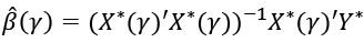Formules_8_str.pdf (10)

The relationship between savings and high-technology export level is demonstrated in Equation 11 which includes one threshold.

Formules_8_str.pdf (11)

It expresses the dependent variable y_it, that is, the current account balance of country i in period t, the error term ε_it, the fixed effects specific to countries u_i, the share of high-technology product export level with exogenous threshold variable π ̃ _it, and the indicator function I_. is doing. In addition, while γ₁ represents the threshold parameters for the savings in the threshold model, X_it represents the vector consisting of control variables.

Table 8. Threshold Regression

Dependent Variable	Coefficient	Standart Error	P>t
Labor	.4185576	.1254176	0.075
Capital	-.4847763	.1383843	0.001
dsavings >38.7299	1.077714	.1254176	0.023

The results of the threshold regression model obtained within the framework of Equation 7 show that savings level which is below the threshold value (Savings ≤ 38.7299) does not affect high-technology export level, whereby savings level above the threshold value (Savings > 38.7299) positively affects the high-technology product export level (Table 8). If the saving level is above threshold, 1% of increase in saving level increases the high-technology product export level by 1.0777%. The interpretation of other two variables of the model is impact of labor on economic growth is positive and 1% percent increase in the employment level (labor) creates 0.42% of increase in the level of economic growth. When capital effect is taken into consideration it is found out that capital has a negative impact on economic growth. 1% of increase in the level of capital creates 0.48% of decrease in the level of economic growth. Although this result related to capital effect is opposite of the Solow model hence, we choose gross capital formation as capital it can be accepted as the investment in physical capital may lead an increase in the economic growth for the subsequent terms even though it has a negative effect for the recent term.

Discussion

This paper is the third research of the series on the high-tech export led growth of the author. The first paper concluded that the HTX level does not have any impact on the economic growth of developing countries. In the second paper it is proved that HTX has a positive impact on economic growth for developed countries, and this was not an unforeseen result. This third paper has been written in order to find out the savings level that is necessary to achieve the HXT export-led growth. Increasing the GDP per capita is the main aim of developing countries for the initial stages of development. After a certain point, some of the countries set their strategies to achieve economic development based on technology such as Korea and China. If we focus on China, we see that they use the advantage of their labor force and produce labor-based products at the initial stage of their development; after achieving a certain level of savings, they have started to invest in technology. For China, between the years 1960–1964, the average gross domestic savings (GDS) per GDP is 22.9%, for the same period gross domestic investments (GDI) per GDP is 22.2%, and GDP per capita is 79.2 USD. For the years 2010–2015, GDS per GDP increased to 52.39%, and for the same period GDI per GDP increased to 45.77%, and GDP per capita increased to 6.523 USD. Another important indicator for assessing the strategy of China is the number of patent applications. The eldest data is from 1985, and the patent application number of China was just 4,065 and this was just 0.62% of the world’s total. For the year 2020, the patent application number of China has reached 1,344,817 and this is 58.4% of the world’s total patent application number. In summary, China is the perfect example for tripartite papers of the author on the HTX-led growth. When it comes to the development aspect, it is observed that HDI (Human Development Index) of China increased from 0.145 in 1960 to 0.768 in 2021. This also indicates that as well as economic growth China achieved economic development with the economic strategies that they imposed.

After examining the high-technology export-led growth for developing and developed countries, with the first two papers, this third one aims to test the impact of the high-technology export level on economic growth with the help of a casualty test as the first step. It is concluded that economic growth and HTX have a bidirectional casualty relationship for 16 countries that have the highest high-technology export levels.

As the second stage of the empirical analysis, threshold regression is applied to test the necessary savings level for providing the high-technology export-led growth. The model that is set to test the mentioned savings level is based on the Solow growth model. It is concluded that a savings level that is below the threshold value (Savings ≤ 38.7299) does not affect the high-technology export level whereas above the threshold value (Savings > 38.7299) it positively affects the high-technology product export level. It is obvious that there are many factors that affect HTX, but for the initial stage a certain level of savings and a strategy based on the HTX-led growth is a must. This result should guide policymakers in the way that 38.73% savings level should be achieved in order to make investments for high-technology products via increasing research and development expenses and patent numbers. With this paper, the level of savings required for countries aiming to grow based on the high-technology product exports has been revealed. This is the first paper in the literature that calculates the savings level that is necessary for the HTX-led growth.

Conclusion

Development, beyond economic growth, requires a change in the economic and socio-cultural structure. Socio-cultural and political evidence of development may be accepted as the high schooling rate, the high rate of female employment, the absence of child labor, the provision of social discipline, the elimination of abuse of authority, such as corruption, and providing opportunities to supporters. On the other hand, the very rapid technological developments experienced throughout the world for the last two decades, and the production and export of high-tech products is handled as an indicator of economic development. As the last aspect, the theorems on foreign trade exhibit that foreign trade supports the development of countries by triggering competition and leading specialization in the sectors in which production factors are abundant thus increasing productivity, by leading to technology transfer. Technological backwardness stands out as a common feature of underdevelopment. The main reason for poverty, which can be considered in common, is that developing countries do not have sufficient capital accumulation and, accordingly, they cannot make progress at their technology level due to their inability to allocate sufficient resources for research and development activities. By combining all theoretical backgrounds, savings which lead to an increase in technology levels of countries, and by producing and exporting high-technology products, an achieving economic growth and development targets is the main underlying idea of this paper. Two-stepped analysis is applied to achieve the target of the paper by taking sixteen countries – Hong Kong SAR, China, Singapore, Malaysia, Vietnam, Korea Rep., Malta, Kazakhstan, Israel, Iceland, Thailand, Ireland, France, Netherlands, United Kingdom, and Norway – which have the HTX level over world’s average. First, it is examined whether the high-technology product export level has a positive impact on economic growth or not. After finding out there is a bidirectional casualty relationship between economic growth and the high-technology product export level, threshold regression is applied to analyze, at which savings point countries can achieve a satisfactory high-technology product export level. The results of the threshold regression model obtained within the framework of Equation 7 show that the savings level which is below the threshold value (Savings ≤ 38.73) does not affect the high-technology export level, whereby above the threshold value (Savings > 38.73) it positively affects the high-technology product export level. If the savings level is above the threshold, 1% of increase in the savings level increases the high-technology product export level by 1.078%. Achieving this result makes this paper the first one in the literature that calculates the savings level that is necessary for the HTX-led growth. Although borrowing from banks and institutions like World Bank and IFC creates resources for investments in technology, the debt crisis that has been experienced by many countries, demonstrated the importance of savings once more.

Ultimately, it is thought that the study reveals a very concrete output for the countries that aim to develop through the export of high-tech products and plan to achieve this by saving as a strong resource. As it was mentioned at the discussion part in detail, countries like China, which change their strategy on the HTX-led growth after reaching a certain level of savings, may be the ones that other counties can learn from. This paper is limited with just exploring the savings level which leads to the HTX-led growth. In the next research, the structure of savings may be investigated: Which source of savings – such as households or central government budget or enterprises – leads to the HTX-led growth the most?

Resourses

Aghion, P., Comin, D., Howitt, P. et al (2016). When Does Domestic Savings Matter for Economic Growth?. IMF Economic Review 64, 381–407. https://doi.org/10.1057/imfer.2015.41

Alzghoul, A., Al_kasasbeh, O., Alsheikh, G., & Yamin, I. (2023). The Relationship Between Savings and Investment: Evidence From Jordan. International Journal of Professional Business Review, 8(3), e01724. https://doi.org/10.26668/businessreview/2023.v8i3.1724

Braunerhjelm, P.& Thulin, P. (2008). “Can countries create comparative advantages? R&D expenditures, high-tech exports and country size in 19 OECD countries, 1981–1999”. International Economic Journal, 22(1), 95–111. https://doi.org/10.1080/10168730801887026

Chang W.W. (1970). “The Neoclassical Theory of Technical Progress”. The American Economic Review 60 (5): 912- 923

Demir, O. (2018). Does High Tech Exports Really Matter for Economic Growth a Panel Approach for Upper Middle-Income Economies . AJIT-e: Academic Journal of Information Technology , 9 (31) , 43-54 . oiI: 10.5824/1309-1581.2018.1.003.x

Đidelija, I. (2021). “The Causal Link Between Savings and Economic Growth in Bosn*ia and Herzegovina” South East European Journal of Economics and Business, vol.16, no.2, pp.114-131. https://doi.org/10.2478/jeb-2021-0018

Dumitrescu, E. I. ve Hurlin, C. (2012), “Testing for Granger Non-Causality in Heterogeneous Panels”, Economic Modelling, 29(4), 1450-1460. Doi: 10.1016/j.econmod.2012.02.014

Ekananda, M., & Parlinggoman, D. J. (2017). The role of high-tech exports and of foreign direct investments (FDI) on economic growth. European Research Studies Journal, 20(4A), 194-212. Doi: 10.35808/ersj/828

Fonkam, A. (2023) Determinants of technology-intensive exports: The case of African countries, 1995–2017, African Journal of Science, Technology, Innovation and Development, DOI: 10.1080/20421338.2022.2156026

Han, E. & Kaya, A.A. (2013). Kalkınma Ekonomisi Teori ve Politika. Ankara. Nobel Akademik Yayıncılık.

Harrod R.F (1948). Towards a Dynamic Economics. London. MacMillan Co Ltd.

Hicks J.R. (1963). The Theory of Wages. London.

Gokmen Y. And Turen U. (2013).”The Determinants of High Technology Exports Volume: A Panel Data Analysis of EU-15 Countries”. International Journal of Management, Economics and Social Sciences, 2013, Vol. 2(3), pp. 217 –232

Joshi, A., Pradhan, S. & Bist, J.P. (2019). Savings, investment, and growth in Nepal: an empirical analysis. Financ Innov 5, 39. https://doi.org/10.1186/s40854-019-0154-0

Kabaklarli, E., Duran, M.S., Üçler, Y.T. (2017). The Determinants of High-technology exports: A Panel Data Approach for Selected OECD Countries. Dubrovnik International Economic Meeting. 3(1): 888-900. https://hrcak.srce.hr/187437

Mankiw, N. G. (2010). Makro Ekonomi. Ankara: Efil Yayınevi.

Pesaran H., Smith R. And Im K.S., (1995) ”Dynamic Linear Models For Heteregenous Panels” Working Papers in Economics 9503, Faculty of Economics, University of Cambridge.

Peseran, H. M. (2004), “General diagnostic tests for cross section dependence in panels”. Discussion Paper, No. 1240 August, p. 5. https://doi.org/10.17863/CAM.5113

Sahi̇n, B. (2019). Impact of High Technology Export On Economic Growth: An Analysis On Turkey. Journal of Business Economics and Finance, 8 (3), 165-172. DOI: 10.17261/Pressacademia.2019.1123

Satrovic E. (2018). Economic output and high-technology export: panel causality analysis. International Journal of Economic Studies, 4(3),55-63. https://dergipark.org.tr/en/pub/ead/issue/48248/610778

Seung-Hoo Yoo (2008) “High-technology exports and economic output: an empirical investigation”, Applied Economics Letters, 15:7, 523-525, Doi: 10.1080/13504850600721882

Sevcan Güneş, Sinem Pınar Gürel, Duygu Yolcu Karadam, Tuğba Akin. (2020). “The Analysis Of Main Determinants of High Technology Exports: A Panel Data Analysıs”. Kafkas Üniversitesi İktisadi ve İdari Bilimler Fakültesi Dergisi 21:242-267. /article-detail?id=878346 The Central and Eastern European Online Library. http://doi.org/10.36543/kauiibfd.2020.012.

Seyoum, B. (2004). The role of factor conditions in high-technology exports: An empirical examination. The journal of high technology management research, 15(1), 145-162. https://doi.org/10.1016/j.hitech.2003.09.007

Singh, T. 2019b. “Saving–Investment Correlations and the Mobility of Capital in the OECD Countries: New Evidence from Cointegration Breakdown Tests.” The International Trade Journal 33 (5): 385–415. doi:https://doi.org/10.1080/08853908.2019.1592727.

Sojoodi, S., Baghbanpour, J. The Relationship Between High-Tech Industries Exports and GDP Growth in the Selected Developing and Developed Countries. J Knowl Econ (2023). https://doi.org/10.1007/s13132-023-01174-3

Solow, R. M. (1957). Technical Change and Aggregate Production Function. The Review of Economics and Statistics, 39(3), 312–320.

Stolper W. F. And P. Samuelson (1941), Protection and Real Wages, H. S. Ellis, L. Z. Metzler (eds) 1966. Readings in the Theory of International Trade, London: George Allen and Unwin.

Şahin, L. and Şahin D. K. (2021). “The Relationship Between High-Tech Export and Economic Growth: A Panel Data Approach for Selected Countries”, Gaziantep University Journal of Social Sciences 20(1): 22-31. https://doi.org/10.21547/jss.719642

Tarlok, S. (2022) Saving-investment correlations and the financial globalization of the BRICS countries, Applied Economics, 54:20, 2257-2274, Doi: 10.1080/00036846.2021.1912280

Tebaldi, E. (2011). The Determinants of High-Technology Exports: A Panel Data Analysis. Atlantic Economic Journal 39, 343–353 (2011). https://doi.org/10.1007/s11293-011-9288-9

Telatar, O. M., Değer, M. K. ve Doğanay, M. A. (2016). “Teknoloji yoğunluklu ürün ihracatının ekonomik büyümeye etkisi: Türkiye örneği (1996: Q1-2015: Q3)”, Atatürk Üniversitesi İktisadi ve İdari Bilimler Dergisi, 30(4): 921-934. https://dergipark.org.tr/tr/download/article-file/315523.

Usman, M. (2017).Impact of High-Tech Exports on Economic Growth: Empirical Evidence from Pakistan,Journal on Innovation and Sustainability, Vol. 8 (1), 91-105. Doi: https://doi.org/10.24212/2179-3565.2017v8i1p91-105

Yılmaz E.G. (2020). The Effect of TFP, Patent Applications and ICT Exports on Per Capita Income in OECD Countries. Interdisciplinary Public Finance, Business and Economics Studies Volume III. Ed. Akıncı A. 225-237. Berlin. Peter Lang.

Yılmaz E.G and Dura Y.C. (2021). Yüksek Teknolojili Dış Satım ve İhracata Dayalı Büyüme Hipotezi Boyutundan Ekonomik Büyüme. ‘Journal of Science-Technology-Innovation Ecosystem’. 2(2), 99-109. http://bityed.dergi.comu.edu.tr/dosyalar/Bityed/cilt-2-sayi-2.pdf

Web Resources

Ceicdata, (2022). https://www.ceicdata.com/en/indicator/china/gross-savings-rate.

Worldbank. (2022). Total investment (% of GDP) - TCdata360 (worldbank.org).

Worldbank. (2022). Gross domestic savings per GDP. https://data.worldbank.org/indicator/NY.GDS.TOTL.ZS

Worldbank. (2022). High-technology exports (% of manufactured exports. https://data.worldbank.org/indicator/TX.VAL.TECH.MF.ZS