Ekonomika ISSN 1392-1258 eISSN 2424-6166

2025, vol. 104(1), pp. 88–102 DOI: https://doi.org/10.15388/Ekon.2025.104.1.5

Do Green Bonds Impact Sustainable Development? An Empirical Analysis

Göksel Karaş*
Kutahya Dumlupinar University, Kutahya, Turkiye
Email: goksel.karas@dpu.edu.tr
ORCID ID: https://orcid.org/0000-0003-4091-1258

Hakan Celikkol
Kutahya Dumlupinar University, Kutahya, Turkiye
Email: hakan.celikkol@dpu.edu.tr
ORCID ID: https://orcid.org/0000-0001-9345-1596

Abstract. Trying to meet unlimited human needs with limited resources causes production activities to deplete or pollute natural resources. Ensuring the sustainability of natural resources and the environment is essential to leaving a livable world for future generations. The concept of sustainable development, which emerged from this attitude, has been on the agenda of many countries, especially supranational organisations, especially in recent years. Based on this, the present study aims to examine the impact of green bonds issued worldwide on sustainable development with the help of panel data analysis for 17 countries that issued the most GBs in the period of 2014–2022. In the study, fixed effect, random effect and GMM tests were applied. Empirical findings show that GB issuances positively affect the environmental performance, while the development levels of countries have a negative effect. The findings also show that the impact of COVID-19 positively affects environmental performance. In the selected countries, trade openness was not found to affect environmental performance significantly.
Keywords: sustainable development, green bonds, developed countries, panel data analysis.

___________

* Correspondent author.

Received: 20/09/2024. Revised: 06/12/2024. Accepted: 05/01/2025
Copyright © 2025 Göksel Karaş, Hakan Celikkol. Published by Vilnius University Press
This is an Open Access article distributed under the terms of the Creative Commons Attribution License, which permits unrestricted use, distribution, and reproduction in any medium, provided the original author and source are credited.

1. Introduction

The rapid development in the global economy has brought about significant environmental degradation which becomes more apparent with every passing year. According to the World Bank data, the world GDP, which was 1.36 trillion dollars in 1960, has reached 105.44 trillion dollars. While this means that production is increasing worldwide, it also means that natural resources are being depleted rapidly. Therefore, problems related to economic growth and sustainable development are essential issues that attract the attention of almost all countries (Cuaresma et al., 2013). Environmental degradation and environmental concerns, among the most critical problems regarding the achievement of sustainable development, have been in the list of the topics of major interest to academics, especially in recent years, in the pursuit to achieve the sustainable development goals (SDGs) emphasised by the United Nations Development Program (UNDP). In the Brundtland Report, sustainable development is defined as development which meets the needs of the present without compromising the ability of future generations to meet their own needs. This definition emphasises equality between generations and the efficient and effective use of resources (Carvalho, 2001; Munier, 2005).

One of the most important factors of environmental degradation is excessive energy consumption and greenhouse gas emissions from fossil fuels (Saha and Maji, 2023). For this reason, the EA Sustainable Development Scenario (SDS) aims to reduce the fossil fuel use by 40% by 2030 and increase the share of renewable energy in the total energy supply to 60%. At the same time, this target is also compatible with the provisions of the Paris Agreement regarding global warming to be below 2°C in the 21^st century (Tolliver et al., 2020). However, in order to achieve this target, a financing of 55 trillion dollars is needed for activities related to environmentally sensitive investments by 2035 (IEA, 2014). Since the traditional financing methods insufficiently fund green projects, the concept of green finance has been developed in this regard.

Green finance is vital in the global financial system as it focuses on investing in projects necessary for environmental sustainability and promoting technologies with low carbon footprints. It is considered an essential innovation in the financial system which aims to promote sustainable growth and address social and environmental challenges. In this context, financial instruments are expected to be critical to achieving the United Nations Sustainable Development Goals by 2030 (Alamgir and Cheng, 2023). Green finance is compatible with the principles of sustainable development. It emphasises the interdependence between human life and the environment. There is a close relationship between green finance and the low-carbon economy. The basis of green finance is to protect the environment and ensure sustainable development by considering potential environmental impacts in making investment and financing decisions (Lee, 2020). Green finance covers various financial instruments, such as green loans, green bonds, green stock indices, green development funds, insurance, carbon finance and policy incentives (Alamgir and Cheng, 2023).

Green bonds (GBs) are one of the green finance products used to support environmentally sensitive or green activities. Globally, green finance applications are dominated by GBs that can provide the necessary financing for green investments by managing expenditures between current and future generations. The issuance of GBs reduces greenhouse gas emissions by implementing environmentally sensitive projects. They can act as a bridge between the financing requirements needed for green projects and funders (Fatica and Panzica, 2021). GBs are defined by the International Capital Markets Association (ICMA) Green Bond Principles (GBP) as “any bond instrument whose proceeds will be used solely, in whole or in part, to finance or refinance new and/or existing eligible Green Projects” (ICMA, 2018). In recent years, there has been a significant increase in the use of green bonds as a financial instrument. The proceeds of these bonds are allocated to financing environmentally friendly and climate-sensitive projects such as renewable energy initiatives, green buildings, resource conservation and sustainable transportation. Additionally, GBs allow governments and other institutions supporting their issuance to encourage the flow of capital to the priority sectors with the objective to achieve public policies and goals such as climate change mitigation and adaptation (Thompson, 2021). GBs and their impact on the environmental situation can be linked to financing sustainable projects, reducing the carbon footprint, increasing environmental awareness, protecting the ecosystem, and transitioning to a green economy. GBs are used to finance environmentally friendly projects such as renewable energy, energy efficiency, sustainable transportation, water management, waste recycling, and protection of natural resources. These projects positively change environmental impacts by reducing carbon emissions and ensuring a more efficient use of natural resources. GBs accelerate the transition to a low-carbon economy. For example, the financing of environmentally friendly renewable energy projects reduces the dependence on fossil fuels. This directly contributes to combating climate change by reducing greenhouse gas emissions. The issuance of GBs draws attention to environmental sustainability issues and increases investors’ awareness of environmentally friendly financing. Investors turn to these bonds by making environmental impact a priority. Investments in projects aimed at protecting natural resources support the protection of biodiversity and the sustainability of ecosystems. GBs accelerate the implementation of environmentally friendly economic models. This ensures both the reduction of environmental damage in the short term and the establishment of a balance between economic growth and environmental sustainability in the long term.

The European Investment Bank (EIB) made the first GB issuance in 2007, and then the World Bank (WB) followed with its own issuance in 2008. The issue created by the EIB was under the name of the climate awareness bond and was worth 807 million USD, while the issue made by the WB was under the name of GB and was worth 2.3 billion Swedish Kronor. Since 2008, the WB has made over 200 GB issuances in 28 different currencies, amounting to approximately 18 billion USD (World Bank, 2023). As of the end of 2023, the total GB issuance in the world was estimated as 2.8 trillion USD (Climate Bonds Initiative, 2024). Although this figure is well behind the target, when the development of the GB issuance is examined, it is seen that it will be one of the critical financial instruments in the future. Another important issue regarding the ecological footprint is the COVID-19 pandemic. In fact, due to the pandemic which affected most countries during this period, countries experienced a quarantine process. During this period, production in most sectors either stopped or slowed down. Based on this, it can be stated that there was an ecological recovery in the world during the periods when quarantine was being applied. This situation was modelled by using a dummy variable in the study.

Development is the process of a country reaching a high(er) economic, social and technological development level. However, this level of development can cause side effects, such as intensive use of natural resources and environmental destruction. The increase in the developed countries’ consumption rates shows a strong correlation between the ecological footprint and the level of development. As stated in the studies of Turner et al. (2007), the ecological footprint per capita in industrialised countries is higher than in low- and middle-income countries. At the same time, an increase in the production amounts of countries increases environmental degradation. In addition to the level of development, which is one of the factors causing an increase in the production of countries, foreign trade is another factor. As the foreign trade rates of countries increase, the need for more production will arise, which will cause more environmental degradation. In fact, Abdeel-Farooq et al. (2017) and Khan et al. (2022) used per capita income and trade openness rates as development indicators in their studies and stated that per capita income and trade openness have a negative effect on environmental performance. According to Saha and Maji (2023), highly developed countries negatively impact the environmental performance more than developing countries. At the same time, it has been found that trade openness also has a negative impact on the environmental performance. Therefore, there is a significant relationship between the development levels of specific countries, their trade openness, and ecological footprints.

Since GBs were first issued in 2008, academic studies on their effects have generally been conducted in recent years. When the studies in the literature are examined, the effects of GBs on sustainable development are generally discussed. At the same time, some theoretical studies on GBs in the literature are also available. Among the empirical studies, some researches (Abdeel-Farooq et al., 2017; Tolliver et al., 2020) focus on the effects of renewable energy production on environmental performance, while others (Miroshnychenko et al., 2017; Ren et al., 2020; Zhou et al., 2020; Li and Gan, 2021; Tran, 2021; Mamun et al., 2022; Fang et al., 2022; Khan et al., 2022; Meo and Abd Karim, 2022; Xiong and Sun, 2023) focus on the effects of green finance practices on environmental sustainability. Relatively few studies in the literature focus on the impact of GBs on factors such as sustainable development and environmental degradation. Ehlers et al. (2020) and Sinha et al. (2021) found that environmental and social sustainability decreased on average in the first years following the issuance of GBs but increased later on. Benlemlih et al. (2022) found that, on the contrary, there was no significant decrease in carbon emissions among GB issuers in the short term, while, in the long term, there was a decrease in CO₂ emissions. The study by Kant (2021) concluded that 200 corporate GBs issued did not significantly affect carbon emissions. Similarly, in the study conducted by Bukvic et al. (2023), they examined the relationship between GB issuances and CO₂ emissions in the EU-27 countries in the period between 2013 and 2017 to investigate the validity of the theory that “GBs reduce carbon emissions by financing environmentally friendly projects.” The study concluded that, despite the dramatic increase in GB issuances from €5 billion in 2013 to €75 billion in 2017, there was a slight decrease in total and per capita CO₂ emissions of 3.7% and 4.6%, respectively, and no significant relationship was found between GB issuances and CO₂ emissions. Fatica and Panzica (2021) conducted a study on 1,105 entities issuing GBs. They concluded that green issuers decreased the carbon intensity of their assets after borrowing in the green segment. Similarly, the study by Chang et al. (2022) concluded that green financing increased the environmental quality in specific segments of the data distribution in eight of the 10 countries that issued the most GBs. In another study, Saha and Maji (2023) concluded that GBs reduced carbon emissions for developing countries in 44 countries between 2016 and 2020, while the same effect weakened for developed countries. Alamgir and Cheng (2023) found that GBs had a positive and significant relationship with renewable energy production in 67 countries during the period of 2007–2021, while emissions had a negative relationship with GBs.

The study aims to determine the impact of GB issues on sustainable development with the help of panel data analysis by answering the research questions (RQ) stated below.

RQ1: What is the general impact of GB issues on ecological footprint?

RQ2: How does higher development affect the ecological footprint?

RQ3: How do commercial concerns affect the ecological footprint?

The study applied panel fixed effects, random effects, and Generalized Method of Moments (GMM) tests for 17 countries that issued the most GBs between 2014–2022. A country limitation is thus involved in the study. Although the first GB issuance was made in 2007, there has not been a regular issuance every year since then. Therefore, when the countries regularly issuing GBs annually are examined, the countries with the highest time interval are 17 developed countries. Based on this, the study sample consists of 17 selected developed countries. The study established a model in which the ecological footprint was the dependent variable indicator of sustainable development, and GB issues, the human development index, trade openness and a dummy variable, which is used to analyse the effect of COVID-19, were independent variables. The studies mainly used CO₂ emissions and the ecological footprint as sustainable development indicators. Independent variables differ under the common roof of green finance. As observed in the literature review, the studies mainly focused on the impacts of variables, such as green finance, renewable energy and energy consumption on sustainable development. The study aims to contribute to the literature in two points. First, by departing from prior works, which only provide some country-specific evidence of the impact of the GB on the ecological footprint, this study investigates the GB ecological footprint relationship for 17 countries which have issued the most GBs after initiating the implementation of the Paris Agreement, adopted in 2015. Second, unlike most of the prior works which examined the effects of GBs on the ecological footprint on a standalone basis, we provide the first evidence that the developed countries’ sustainable development moderates the GB and ecological footprint nexus.

The rest of the paper is organised as follows. Section 2 briefly describes the methodology. Section 3 reports empirical results from the Panel regression and GMM tests, and policy implications are summarised in the final section.

2. Methodology and Data

According to the data requirements, the present study uses the traditional panel data models such as the fixed effect model (FEM) and the random effect model (REM) as well as the generalized method of moments (GMM) model. With a small sample size, FEM, REM, and GMM are the most suitable methods for analytical estimation (Gujarati, 2003). In addition, Hausman’s specification test (Hausman, 1978) determines which model is suitable for analysis. If the P value of Hausman’s specification test is less than 0.5 (P<0.5), the fixed effect model is the best option. Otherwise, the random effect model is the best option. The traditional fixed effect, random effect and GMM models are most suitable, especially if the sample panel data is small, covering the period 2014–2022 for seventeen countries, which is the case in the present study. In addition, we complement the fixed effect and random effect estimators by using the robust least squares technique so that to ensure the robustness of the study’s results.

2.1. Methodology

In a study conducted to determine the impact of GBs, which are used to finance environmentally friendly projects serving the objective to prevent or reduce environmental degradation, while focusing on sustainable development, annual data between 2014 and 2022 were used. The model created within the scope of the study is given below.

efit=β₀ + β₁lngb_(i(t–1)) + β₂lnhdiit + β₃lnopenit + β₄dummyit + εit (1)

In the Equation, ‘ef’ represents the ecological footprint, ‘gb’ stands for the natural logarithm of GB issues, ‘hdi’ denotes the natural logarithm of the human development index, ‘open’ is the natural logarithm of trade openness, ‘dummy’ represents a variable created to measure the impact of the COVID-19 pandemic, ‘β’ is used for the coefficient of the relevant variables, ‘ε’ serves as the error term, ‘i’ stands for the cross-section units, and ‘t’ denotes the time interval. It was also concluded that adding the GB issues variable to the model with a delay of one year would be meaningful since the effects of investments manifest themselves in more than one year.

Among the variables in the Equation, GB issues are expected to have a negative effect on the ecological footprint. As GBs are used to finance environmentally friendly projects, they are expected to reduce environmental degradation and positively affect sustainable development. Another independent variable, the human development index, which represents development, is also expected to have a negative effect on the ecological footprint. As the development levels of countries increase, it is expected that environmentally friendly projects will not be experiencing financing problems, and that their sensitivity to this issue will be high, thus reducing the ecological footprint. The final independent variable, the trade openness data, is expected to affect the ecological footprint positively. Since the increase in the trade volumes of countries means an increase in production amounts, the economic purpose comes to the fore rather than environmental sensitivity. In this case, environmental degradation is expected to increase even more. Based on this, the hypotheses to be tested in the study are formed as follows:

Hypothesis 1: GB issues have a reducing effect on the ecological footprint.

Hypothesis 2: The development levels of countries have an increasing effect on the ecological footprint.

Hypothesis 3: The level of trade openness of countries has an increasing effect on the ecological footprint.

The model estimation phase was started after testing the stationarity of the series used in the study. For this purpose, Breusch Pagan’s (1980) test was applied to determine the most appropriate method for estimating the Pooled Least Squares and the panel regression methods. The Pooled Least Squares method is tested against the random effects model in the test. The null hypothesis is that the variance of the unit effects is zero; that is, the Pooled Least Squares method estimation is the most appropriate (Breusch and Pagan, 1980). After determining that the estimation with the panel regression model is appropriate, it is necessary to determine whether the equations have fixed or random effects. For this purpose, the Hausman (1978) test was applied. The null hypothesis in the test is that there is no correlation between the units; that is, that random effects are manifested (Hausman, 1978). Basic assumption tests, namely, heteroscedasticity and autocorrelation, were performed based on the estimation method through the random effects model obtained from the Hausman (1978) test results. Levene-Brown-Forsythe’s tests were performed for heteroscedasticity, and Bhargava, Franzini and Narendranathan Durbin-Watson and Baltagi Wu LBI tests were used for autocorrelation. In econometric analyses, the heteroscedasticity problem is mainly encountered in studies conducted with cross-sectional data. The situation where the variance changes according to the units within the cross-sectional units is called heteroscedasticity (Yerdelen Tatoğlu, 2016). The heteroscedasticity problem in the random effects model is analysed by using the Levene-Brown-Forsythe test. According to the test proposed by Levene (1960), robust estimates are also presented in cases where the normal distribution assumption is not realised (Yerdelen Tatoğlu, 2016). The Levene-Brown-Forsythe test null hypothesis is that no heteroscedasticity problem exists according to the units (Greene, 2003). Due to the usage advantages of the Durbin-Watson test statistic, the Durbin-Watson autocorrelation test statistic was developed by Bahrgava, Franzini and Narendranathan (1982) using the AR(1) model in order to test autocorrelation in both fixed and random effect models. Accordingly, the null hypothesis is that there is no autocorrelation between units (Bhargava et al., 1982). In addition to the Durbin-Watson test statistic developed by Bhargava et al., the Locally Best Invariant (LBI) test developed by Baltagi-Wu (1999) was also applied. The LBI test can be used for both fixed and random effect models. It can also be used for unbalanced models. The null hypothesis is established as no autocorrelation (Baltagi and Wu, 1999).

2.2. Data

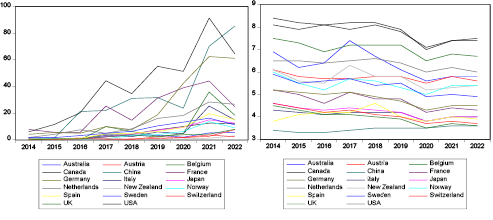
Ecological footprint was used as an indicator of sustainable development and a dependent variable; the data related to ecological footprint were obtained from York University, National Footprint and Biocapacity Accounts. The GB issue amounts, used as independent variables, were obtained from the Climate Bonds Initiative database, the development indicator human development index data were sourced from the United Nations Human Development Index database, while the trade openness rates were retrieved from the World Bank database. Figure 1, showing the development of the series, is given below.

Green Bond Issues Ecological Footprint

Trade Openness HDI

Figure 1. Development of series by country over the years

Note. Adapted from York University, National Footprint and Biocapacity Accounts, Climate Bonds Initiative, United Nations and World Bank databases, (2024).

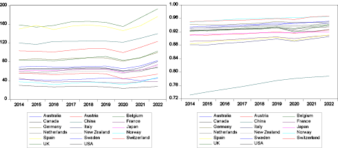
Six components were used to calculate the ecological footprint: the carbon footprint, the agricultural land footprint, the forest footprint, the structured area footprint, the fishing area footprint, and the pasture footprint. A high ecological footprint value means that sustainability is negatively affected. From this point on, as seen in Figure 1, the country with the highest ecological footprint based on the horizontal sections in the panel is the USA, with 7.83. It is followed by Canada with 7.80, Belgium with 7.03, the Netherlands with 6.34, and Australia with 6.32.

When GB issuances are examined, the USA, which has issued GBs worth over 10 billion dollars, is again in the first place whereas China comes in the second place, Germany follows in third place, France is in the fourth place, and the Netherlands finds itself in the fifth place. The striking point here is that the ecological footprint of the USA is still high despite having the highest GB issuance. This can be interpreted as an assumption that the GB issuances in the USA are not having the expected effect. China, which is given the second place and which has the lowest ecological footprint, is the country that can be interpreted as denoting the effectiveness of GB issuances.

When the HDI scores are examined, it is evident that the development rates of all the investigated countries except for China are close to one. This can be interpreted as a point that the countries in the panel are denoted by high human development.

When the trade openness rate calculated as the share of the total trade volume in GDP is examined, the country with the highest value in terms of trade openness is Belgium, with 165.45%. Meanwhile, Spain comes second with 156.33%, China is third with 125.03%, and Austria ranks fourth with 106.89%. The USA is in the final position with 26.90%. This situation is somewhat remarkable for the USA, which is one of the leading advocates of neoliberal policies towards re-establishing the functioning of the market economy and making free trade the dominant policy in international trade.

3. Results and Discussion

The study examined the effects of GB issues on sustainable development for the 17 countries issuing the most GBs with the help of panel regression analysis. In this context, firstly, Breusch Pagan’s (1980) test was applied in order to determine which method would be the most appropriate for estimation between the Pooled Least Squares method and the panel regression method. The results of the Breusch Pagan (1980) analysis are given in Table 1.

Table 1. Breusch Pagan (1980) test results

Note: * shows significance at the 1% level.

According to Table 1, the null hypothesis was rejected at a significance level of 1% for the model tested within the study’s scope. It was concluded that the estimate should be obtained by using the panel regression method. Then, the Hausman (1978) test was applied to decide whether the model would be appropriate to estimate with fixed or random effects. The results of the Hausman (1978) test are shown in Table 2.

Table 2. Results of Hausman (1978) Test

According to the results in Table 2, the null hypothesis cannot be rejected. It was concluded that the random effects model was more appropriate as an estimation method. The estimation was continued by using the random effects model, and heteroscedasticity and autocorrelation tests were conducted to determine whether the estimated models meet the basic assumptions. Instead of carrying out the ANOVA on absolute deviations from the mean of each group, it is done on the absolute deviations of observations from either the median or the 10% trimmed mean of each group. Three test statistics are calculated by using the Levene-Brown-Forsythe test. These test statistics are W₀, W₅₀, and W₁₀. If the calculated test statistics are greater than 0.05, the null hypothesis of no heteroscedasticity problem between the units is rejected. In order to determine the autocorrelation between the units in the model, the Bhargava, Franzini and Narendranathan test and the Baltagi-Wu LBI test were applied. Suppose the Durbin-Watson test statistics calculated as a result of the test are close to 2. In that case, this indicates that there is no autocorrelation problem, and if the test statistics are found to be less than 1, this indicates that there is an autocorrelation problem (Bhargava, Franzini, and Narendranathan, 1982; Baltagi and Wu, 1999).

The results of the Levene-Brown-Forsythe test for heteroscedasticity and the Lagrange multiplier test for autocorrelation are given in Table 3.

Table 3. Results of the Heteroscedasticity and Autocorrelation Test

In the findings in Table 3, there is no problem with both heteroscedasticity and autocorrelation in the model tested within the scope of the study because the null hypothesis cannot be rejected in both tests.

A balanced panel of 17 developed countries was used in the study. After estimating the fixed and random effect models, Hausman’s specification test was conducted for the decision to use FEM or REM. Based on the Hausman test results, a random effect model was used in the study with a highly significant P value (P>0.5) and a chi-square statistic of 0.53.

In addition, a dynamic panel data analysis type, the ‘Two-Stage Generalized Moments (GMM) Estimator’, developed by Arellano and Bond (1991), was used in the study. The analysis is also known as the ‘Two-Stage Instrumental Variables Estimator’. There are also different versions of the GMM method. The method which Arellano and Bond (1991) used in this study includes some features and conditions. Firstly, this method is used in the panel data; It can be used when T is less than N (T<N). It also requires a linear functional relationship and the presence of an endogenous variable which interacts with its previous values. In addition, it can be valid in the presence of independent variables that are not strictly exogenous and in the presence of autocorrelation and heteroscedasticity depending on the section, although not between the sections (Roodman, 2009). Panel estimation results are given in Table 4.

Table 4. Panel Estimation Results

Note: * and ** show significance at the 1% and 5% levels, respectively.

According to the results of panel fixed effects, random effect and GMM estimation, the effect of explanatory variables, except for trade openness, on the ecological footprint in developed countries is relatively significant. In particular, the results show that GB issues significantly and positively affect the environmental performance indicator ecological footprint in the selected developed countries at 1%. According to the findings, the coefficient of GB issues is negative. Since this means a decreased ecological footprint, GB issues positively affect the environmental performance in the selected developed countries. In other words, a 1% increase in GB issues positively affects the environmental performance by reducing the ecological footprint by 0.1 units. This result shows that GB issues can positively affect the environmental performance, namely, sustainable development, if used within the scope of their purpose. However, although GB export reduces the ecological footprint, this situation cannot be interpreted as having the same effect in the long term when the findings of the studies in the literature are taken into account. There is a possibility that this effect will reverse unless the necessary improvements and arrangements are made in the long term. The low coefficient can be shown as evidence for this situation.

When the relationship between HDI, a development indicator, and ecological footprint is examined, the HDI indicator has a significant and positive effect on the ecological footprint in the selected developed countries at 5% in the fixed effects model and 1% in other models. According to the findings, a 1% increase in the HDI indicator has a negative effect on the environmental performance by increasing the ecological footprint by approximately 9 units. The economic structures of developed countries are based on high consumption, industrialisation, and fossil fuel use, which increase their ecological footprint. However, developed countries tend to reduce their ecological footprint by investing more in environmentally friendly technologies. However, these investments have not yet fully balanced the consumption of natural resources and the overall impact on the environment. These findings indicate that countries need to re-evaluate their development strategies regarding environmental sustainability. The development of environmentally friendly technologies along with implementation of sustainable development policies can play an essential role in reducing the ecological footprint. The findings confirm this situation.

No statistically significant effect of the trade openness of countries on the environment could be determined. It can be stated that this result is due to the lack of global standards regulating the impact of trade on the environment. At the same time, it can be stated that the indirect effects of trade on the environment are not seen in the short term, and the study’s time constraints make the result insignificant.

In addition, the dummy variable added to the model to determine the impact of the COVID-19 pandemic on environmental performance has a statistically significant effect on the environmental performance at the level of 1%. According to the findings, the quarantines implemented during the COVID-19 pandemic and the decreases in production have a 0.3 unit reducing effect on the ecological footprint. Therefore, it can be stated that the pandemic period positively affects the environmental performance. The findings obtained in the study support each other with the findings obtained in the studies conducted by Ren et al. (2020), Li and Gan (2021), Sinha et al. (2021), Khan et al. (2022), Chang et al. (2022), Meo and Karim (2022), Saha and Maji (2023) and Alamgir and Cheng (2023) in the literature.

4. Conclusion

The study examines the impact of GBs on sustainable development in the context of the countries issuing the highest volume of GBs. We used GB data from 2014 to 2022 and examined the impact of GBs on the ecological footprint. Traditional panel data models, fixed and random effects estimators, and the GMM method were used. The empirical findings largely confirm the results of previous studies in the field. Our results show that GB issuances reduce the ecological footprint of the seventeen selected developed countries, i.e., they improve their environmental performance. However, the coefficient of GBs is relatively low. Therefore, for this effect to be sustainable in the long term, countries need to update the necessary legislative infrastructure to encourage the export of GBs and increase the environmental awareness. Otherwise, it seems that the positive effects of GBs on the environment will be meaningless in the long term. In addition, it was established that the development levels of the countries have a negative and significant effect on the environmental performance in these countries. In addition, it was found that the COVID-19 pandemic positively affected the environmental performance. It was also discovered that trade openness rates in the selected countries did not statistically affect the environmental performance. The present study is essential in terms of its results, guiding policymakers in other countries to develop appropriate policies to address environmental problems, starting from developed countries. The results can also signal the governments about the types of industries that should consider environmental performance in renewing existing enterprises or launching new enterprises. Countries and firms with problems in finding financial resources can apply to GBs in this regard, which can be a priority for governments to encourage them. These findings highlight the instrumental role of GBs in promoting sustainable development and emphasise the importance of their implementation, especially in countries aiming to achieve sustainability goals.

Our study has several limitations that should guide future studies on this topic. The study results are valid for the countries we selected and other regions experiencing GB issues. This study focuses on a specific set of countries (the top 17 GB supporting countries). In contrast, varying groupings of economies or regions may significantly impact the estimates.

5. Policy Implications

Considering that natural resources are being systematically destroyed in the world with each passing day, the importance of sustainable development becomes ever more apparent. In order to ensure sustainable development, the number of environmentally sensitive, as well as environmentally friendly investments must undoubtedly be increased. In this regard, necessary regulations must be adopted by both supranational institutions and individual countries. At this point, the problem of financing the investments to be made comes to mind. In order to increase environmentally friendly projects, it is of importance to reduce the obstacles that have emerged or may arise over time for the development of GBs, one of the green financing instruments. Based on the findings of the present study, the following suggestions can be made for the development of GBs:

1. Countries that issue low GBs can follow in the footsteps of other countries.

2. In addition to the necessary tax incentives, public expenditures should be channelled to the relevant areas through fiscal policies.

3. While GB indexes are currently calculated on 24 country stock exchanges regarding GBs, these indexes should be developed for other countries as well to promote GB issues.

4. GB issuance should be facilitated by providing more incentives in regions and countries where air quality is poor and environmental degradation is high.

5. Since GB, on average, significantly reduces the ecological footprint in the selected countries, regulators and policymakers should follow a strict policy on the maximum use of GBs.

6. Developed countries may consider some other GF instruments besides using GBs to achieve sustainability goals.

References

Adeel-Farooq, R. M., Bakar, N. A. A., Raji, J. O. (2017). Green field investment and environmental performance: a case of selected nine developing countries of Asia. Environmental Progress & Sustainable Energy, 3(3), 1085–1092. https://doi.org/10.1002/ep.12740.

Alamgir, M., Cheng, M. C. (2023). Do green bonds play a role in achieving sustainability?. Sustainability, 15, 1–27. https://doi.org/10.3390/su151310177.

Baltagi, B. H., Wu, P. X. (1999). Unequally Spaced Panel Data Regressions With Ar(1) Disturbances. Econometric Theory, 15(6), 814–823. https://www.jstor.org/stable/3533276.

Benlemlih, M., Jaballah, J., Kermiche, L. (2022). Does financing strategy accelerate corporate energy transition? Evidence from green bonds. Business Strategy and The Environment, 32, 878–889. https://doi.org/10.1002/bse.3180.

Bhargava, A., Franzini, L., Narendranathan, W. (1982). Serial Correlation and The Fixed Effects Model. Review of Economic Studies, 49(4), 533-549. https://www.jstor.org/stable/2297285.

Breusch, T. S., Pagan, A. R. (1980). The lagrange multiplier test and ıts application to model specification in econometrics. Review of Economic Studies, 47, 239–253. https://doi.org/10.2307/2297111.

Bukvić, I. B., Pekanov, D., Crnković, B. (2023). Green bonds and carbon emissions: the European Union case. Ekonomski vjesnik/Econviews - Review of Contemporary Business, Entrepreneurship and Economic Issues, 36(1), 113–123. https://doi.org/10.51680/ev.36.1.9.

Carvalho, O. G. (2001). Sustainable development: is it achievable within the existing international political economy context?. Sustainable Development, 9(2), 61–73. https://doi.org/10.1002/sd.159.

Chang, L., Taghizadeh-Hesary, F., Chen, H., Mohsin, M. (2022). Do green bonds have environmental benefits?. Energy Economics, 115, 1–12. https://doi.org/10.1016/j.eneco.2022.106356.

Climate Bonds Initiative (CBI). (2024). Interactive data platform. Retrieved from https://www.climatebonds.net/market/data/#issuer-type-charts.

Cuaresma, J. C., Palokangas, T., Tarasyev, A. (2013). Green growth and sustainable development. Berlin/Heidelberg: Springer. https://doi.org/10.1007/978-3-642-34354-4.

Ehlers, T., Mojon, B., Packer, F. (2020). Green bonds and carbon emissions: exploring the case for a rating system at the firm level. BIS Quarterly Review, Retrieved from https://www.bis.org/publ/qtrpdf/r_qt2009c.htm.

Fang, Z., Yang, C., Song, X. (2022). How do green finance and energy efficiency mitigate carbon emissions without reducing economic growth in G7 countries? Front. Psychol., 13, 1–11. https://doi.org/10.3389/fpsyg.2022.879741.

Fatica, S., Panzica, R. (2021). Green bonds as a tool against climate change?. Business Strategy and The Environment, 30, 2688–2701. https://doi.org/10.1002/bse.2771.

Greene, W. H. (2003). Econometric Analysis (5th ed.). New Jersey: Prentice Hall.

Gujarati, D. N. (2003). Basic Econometrics (4th ed.). Economic series McGraw-Hill international editions: Economic series.

Hausman, J. A. (1978). Specification tests in econometrics, Econometricia, 46(6), 1251–1271. https://doi.org/10.2307/1913827.

ICMA. (2018). Green Bond Principles: Voluntary Process Guidelines for Issuing Green Bonds. International Capital Market Association, Zürich.

IEA (2014). World energy outlook 2014. International Energy Agency, ISBN: 978-92-64-20805-6.

Kant, A. (2021). Practical vitality of green bonds and economic benefits. Review of Business and Economics Studies, 9(1), 62–83. https://doi.org/10.26794/2308-944X-2021-9-1-62-83.

Khan, M. A., Riaz, H., Ahmed, M., Saeed, A. (2022). Does green finance really deliver what is expected? An empirical perspective. Borsa Istanbul Review, 22(3), 586–593. https://doi.org/10.1016/j.bir.2021.07.006.

Lee, J. W. (2020). Green finance and sustainable development goals: the case of China. Journal of Asian Finance Economics and Busisness, 7(7), 577–586. https://doi.org/10.13106/jafeb.2020.vol7.no7.577.

Li, C., Gan, Y. (2021). The spatial spillover effects of green finance on ecological environment empirical research based on spatial econometric model. Environmental Science and Pollution Research, 28, p. 5651–5665. https://doi.org/10.1007/s11356-020-10961-3.

Mamun, M. A., Boubaker, S., Nguyen, D. K. (2022). Green finance and decarbonization: Evidence from around the World. Finance Research Letters, 46(B), 1–7. https://doi.org/10.1016/j.frl.2022.102807.

Meo, M. S., Abd Karim, M. Z. (2022). The role of green finance in reducing CO2 emissions: An empirical analysis. Borsa Istanbul Review, 22(1), 169–178. https://doi.org/10.1016/j.bir.2021.03.002.

Miroshnychenko, I., Barontini, B., Testa, F. (2017). Green practices and financial performance: A global outlook. Journal of Cleaner Production, 147, 340–351. https://doi.org/10.1016/j.jclepro.2017.01.058.

Munier, N. (2005). Introduction to sustainability: Road to a Beter Future. Dordrecht: Springer.

Ren, X., Shao, Q., Zhong, R. (2020). Nexus between green finance, non-fossil energy use, and carbon intensity: Empirical evidence from China based on a vector error correction model. Journal of Cleaner Production, 277, 1–12. https://doi.org/10.1016/j.jclepro.2020.122844.

Roodman, D. (2009). How to do Xtabond2: An Introduction to Difference and System GMM in Stata. The Stata Journal, 9(1), 86–136. https://doi.org/10.1177/1536867X0900900106.

Saha, R., Maji, S. G. (2023). Do green bonds reduce CO2 emissions? Evidence from developed and developing nations. International Journal of Emerging Markets, Retrieved from https://doi.org/10.1108/IJOEM-05-2023-0765. https://doi.org/10.1108/IJOEM-05-2023-0765.

Sinha, A., Mishra, S., Sharif, A., Yarovaya, L. (2021). Does green financing help to improve environmental & social responsibility? Designing SDG framework through advanced quantile modelling. Journal of Environmental Management, 292, 1–13. https://doi.org/10.1016/j.jenvman.2021.112751.

Thompson, S. (2021). Green and sustainable finance: principles and practice. London: Kogan Page Publishers.

Tolliver, C., Keeley, A. R., Managi, S. (2020). Policy targets behind green bonds for renewable energy: Do climate commitments matter? Technological Forecasting and Social Change, 157(C), 1–11. https://doi.org/10.1016/j.techfore.2020.120051.

Tran, Q. H. (2021). The impact of green finance, economic growth and energy usage on CO2 emission in Vietnam – a multivariate time series analysis. China Finance Review International, 12(2), 280–296. https://doi.org/10.1108/CFRI-03-2021-0049.

Turner, B. L., Lambin, E. F., & Reenberg, A. (2007). The emergence of land change science for global environmental change and sustainability. Proceedings of the National Academy of Sciences, 104(52), 20666-20671. https://doi.org/10.1073/pnas.0704119104.

World Bank. (2023). IBRD funding programs, green bonds. Retrieved from https://treasury.worldbank.org/en/about/unit/treasury/ibrd/ibrd-green-bonds#:~:text=The%20World%20Bank%20Green%20Bonds,affected%20people%20adapt%20to%20it.

Xiong, Q., Sun, D. (2023). Retraction Note: Influence analysis of green finance development impact on carbon emissions: an exploratory study based on fsQCA. Environ Sci Pollut Res Int., 18, 61369–61380. https://doi.org/10.1007/s11356-021-18351-z.

Yerdelen Tatoğlu, F. (2016). Panel Veri Ekonometrisi. İstanbul: Beta Yayıncılık.

Zhou, X., Tang, X., Zhang, R. (2020). Impact of green finance on economic development and environmental quality: a study based on provincial panel data from China. Environmental Science and Pollution Research, 27, 19915–19932. https://doi.org/10.1007/s11356-020-08383-2.