Organizations and Markets in Emerging Economies ISSN 2029-4581 eISSN 2345-0037
2024, vol. 15, no. 2(31), pp. 331–355 DOI: https://doi.org/10.15388/omee.2024.15.16
Bank Diversification, Competition and Earnings Opacity
Japan Huynh
Ho Chi Minh City Open University, Vietnam
japan.h@ou.edu.vn
https://ror.org/00tean533
Abstract. The paper explores the impact of bank diversification on earnings opacity. We aim at offering a comprehensive analysis by focusing on four dimensions of diversification: income, assets, funding, and loan portfolios. Using data from Vietnam over the period 2007–2022, we document consistent and robust evidence that increased diversification across all forms mitigates earnings management via discretionary loan loss provisions. To shed further light on this pattern, we examine how the banking complexity and opacity nexus varies with multiple measures of bank competition. We find that more intense competition in the banking system likely accentuates the impact of diversification on bank earnings manipulations. Our findings provide important implications related to bank business models and banking market structures in the era of financial deregulation and innovation.
Keywords: bank diversification, bank opacity, competition, loan loss provisions
Received: 2/4/2024. Accepted: 20/8/2024
Copyright © 2024 Japan Huynh. Published by Vilnius University Press. This is an Open Access article distributed under the terms of the Creative Commons Attribution Licence, which permits unrestricted use, distribution, and reproduction in any medium, provided the original author and source are credited.
1. Introduction
The opacity inherent in banking operations is correlated with a dearth of informative content, rendering the comprehensive scrutiny of bank activities and the evaluation of the efficacy of bank financial disclosures challenging for external stakeholders, namely investors and creditors (Kozubovska, 2017). Observably, banks in general remain more opaque than other non-bank enterprises due to their power to carry complicated financial assets and keep banking items off the balance sheet (Flannery et al., 2013). It is claimed that the opacity of bank earnings could hamper banks’ regulations and market disciplines since it discourages external parties from accurately evaluating bank risk-taking behaviors (Jungherr, 2018). In practical implementation, regulatory initiatives within the banking sector have been promulgated to advocate heightened transparency, augmented disclosure, and more stringent adherence to market discipline, which is notably exemplified in the provisions of frameworks like Basel III (Fosu et al., 2018).
A growing body of literature has examined the incentives and consequences of bank opacity. As a result, previous studies reveal that bank opacity emerges due to some fundamental reasons, such as income-smoothing motivations (Ozili, 2022), regulatory capital requirements (Barth et al., 2017), financing costs (Jin et al., 2018), private information signaling about future prospects (Huang & Ratnovski, 2011), and poor audit quality (Altamuro & Beatty, 2010). In another vein, bank earnings manipulation is found to hurt financial stability, market valuation, and even asset quality of banks (Beatty & Liao, 2011; Cao, 2022; Dang & Huynh, 2023; Jones et al., 2013; Tran et al., 2022).
This study expands on the current literature stream by examining the impact of bank diversification on earnings opacity. Our motivation in this context stems from the proposition that increased diversification leads to greater complexity in bank business models, influencing choices related to bank opacity. This complexity arises from holding intricate financial assets and delaying the reporting of expected losses (Flannery et al., 2013). Furthermore, a business model toward diversification may well signal banks’ risk-taking propensity, hence it could be associated with their approach in earnings manipulation practices (Morgan, 2002). In the literature, bank diversification has been widely demonstrated to significantly shape bank performance and behaviors (Abbas & Ali, 2022; Maghyereh & Yamani, 2022; Moudud-Ul-Huq et al., 2018; Najam et al., 2022); nevertheless, limited understanding exists regarding the variation of earnings opacity in relation to bank diversification. We also deepen our analysis by investigating how increased competition in the banking market drives the impact of diversification on earnings opacity. Competition may accentuate information asymmetry or monitoring pressure caused by diversification of bank operations (Dell’Ariccia & Marquez, 2006; Nickell, 1996), and it is also closely linked to an excuse for managerial expropriation by banks to obscure financial performance information from stakeholders (Data et al., 2011). Hence, it is interesting to discuss whether the association between diversification and earnings opacity depends on bank competition.
We address the objectives mentioned above by employing a panel of commercial banks in Vietnam over the 2007–2022 period. Four dimensions are utilized to capture bank diversification: income, assets, funding, and sectoral loan portfolios. In line with the existing literature, we establish a regression model of loan loss provisions with a range of bank-specific characteristics and macroeconomic factors as explanatory variables that aim to encapsulate the level of informativeness in financial disclosure (Desalegn & Zhu, 2021; Jiang et al., 2016; Tran & Ashraf, 2018). In case the suggested model has a good potential in estimating loan loss provisions, alternatively speaking, the ambiguity of provision estimation is low, then the residuals of the regression model should be small. Thus, this justifies the use of the residuals’ absolute values to capture the informativeness level of financial disclosure and thus bank earnings opacity. Besides, to ensure a comprehensive and consistent conclusion, we use several different measures to reflect bank competition in this study. Using different competition measures could avoid misleading results obtained from each single one that has its own advantages and disadvantages of reflecting competition (Khan et al., 2016).
Vietnam offers an ideal setting for conducting research, given its heavy reliance on the banking system for both operational functioning and economic growth (Dang & Huynh, 2023). Since 2007, when Vietnam joined the World Trade Organization, the banking sector in Vietnam has undergone extensive deregulation and liberalization reforms. These reforms have modified the banking sector landscape, leading to a more competitive environment (Dang & Huynh, 2022). Under the competition pressure, Vietnamese banks have diversified their operations across different segments to maintain profitability, thus increasing the complexity of their business models. They have shifted into non-lending activities, increased non-interest income, and spread their loan portfolios into many economic sectors (Huynh & Dang, 2021). They have also been less reliant on retail deposits that are substituted by other non-deposit funding sources (Dang & Huynh, 2022). Despite various reforms to upgrade the system, the banking sector in Vietnam has still been characterized by opaqueness that is even more severe than those in other emerging economies (Nguyen, 2023). In this context, the Basel III framework that has emphasis on information disclosure and transparency has currently received little interest from regulators and banks themselves.
To date, scant attention has been devoted to examining the connection between diversification and bank opacity. Existing studies, albeit from diverse perspectives, have yielded varied and inconclusive results. Tran et al. (2019) focus on the US banking system and indicate a positive association between bank diversification and earnings manipulation. They also suggest that bank size and dividend policies are crucial factors moderating this association. Lartey et al. (2022) are interested in banks in the UK and document that functional diversification of banks may enhance earnings opacity, but this pattern is only applicable to the short run, which completely contrasts with the long-run perspective. However, these two studies have analyzed the impact of bank diversification on opacity using the samples of developed countries, different from our strategy that pays attention to an emerging market setting. More importantly, our work differs from these two earlier papers in other key dimensions. Prior authors have only examined the dimension of income diversification, through the income structure captured by aggregate non-interest income, while we ask whether banks diversifying across different income, assets, funding, and loan portfolios can alter the earnings management. In this regard, we look into the disaggregated components of each diversification profile, i.e., we decompose bank income, assets, funding, and loan portfolios into various parts for diversification analysis. Besides, beyond exploring whether bank diversification can drive earnings opacity, we examine how competition affects the impact. The studies of Tran et al., (2019) and Lartey et al. (2022) have largely ignored this conditionality under which diversification may influence bank earnings manipulation heterogeneously.
The empirical analysis of this paper contributes to the literature strands on bank diversification and earnings opacity, which have drawn renewed attention as being regarded as reasons for the 2007–2009 financial crisis. We perform our analysis by considering the banking sector in Vietnam – a typical emerging market, in the context that the literature on the present topic is limited and few prior studies are only interested in developed markets (Lartey et al., 2022; Tran et al., 2019). It should be reminded that the level of financial maturity, regulatory backgrounds, and the depth of deregulations and innovations in emerging markets are quite different from those of developed countries; thus, exploring the impact of diversification on opacity in the banking system of the emerging market is worthwhile. Notably, taking a further step than previous studies, in this paper we pursue a comprehensive examination by looking at four dimensions of diversification, including income, assets, funding, and loan portfolios. This approach is novel in the literature. We also provide additional empirical evidence on the moderating role of competition in the diversification-opacity nexus literature, which has been left unaddressed by scholars thus far.
2. Related Literature and Hypotheses Development
The expansion into various segments at diversified banks raises the complexity of their balance sheets (Fosu et al., 2018). On the one hand, this complexity makes their earnings challenging to forecast (Thomas, 2002). On the other hand, extensive operations may require a large board capable of monitoring banks’ activities, which might cause higher agency costs and create opportunities for bank managers to obtain private benefits (Jensen, 1986). In other words, operating under a diversified strategy increases the likelihood of bank managers incapable of effectively monitoring bank activities due to self-serving managerial behaviors (Chen et al., 2011). Moreover, the action of diversifying bank operations could also boost information asymmetry between the bank and its stakeholders (Rodríguez-Pérez & van Hemmen, 2010). In sum, the incentive to distort financial information disclosures could be heightened by bank diversification as a result of weak monitoring and strong information asymmetry. Therefore, we hypothesize the following:
Hypothesis 1A. Diversification within the banking sector exerts a positive influence on the practice of earnings management.
However, the literature also suggests another line that contradicts the one discussed above, thereby claiming that earnings opacity decreases as bank diversification increases. Theories indicate that diversified banks could gain inside information by developing a variety of close relationships with their customers, thus reducing asymmetric information (Boot, 2000). Fllowing the monitoring argument, despite greater complexity and larger size due to banking extensions, bank diversification is suggested to enhance scrutiny from regulatory authorities and rating agencies (Acharya et al., 2006). Based on information mechanisms from these external parties, which could provide outsiders with performance reports of banks to serve their strategic decisions, bank managers should be discouraged from pursuing practices adversely influencing outsiders (Yu, 2008). In light of the above arguments, we develop the following hypothesis:
Hypothesis 1B. Diversification within the banking sector exerts a negative influence on the practice of earnings management.
Motivated by the literature, we anticipate that the influence of diversification on opacity is contingent upon the level of bank competition. The theoretical literature on banking suggests the problem of asymmetric information faced by banks is more severe in a highly competitive banking sector (Dell’Ariccia & Marquez, 2006). The mechanism is that banks collect helpful information, for instance, by setting up close relationships with customers; however, higher competition among banks may damage this relationship or diminish its length. Supporting the hypothesis of asymmetric information, Fosu et al., (2018) have recently documented that operating in more competitive markets induces banks to be more opaque in earnings management. However, contrary to the above, market competition is also suggested to mitigate asymmetric information and lead to greater monitoring. Accordingly, more intense competition signals greater risk (Allen & Gale, 2004), thus enhancing the quality of internal corporate governance as well as the external monitoring disciplines (Nickell, 1996). Offering evidence in favor of this monitoring hypothesis, Jiang et al. (2016) reveal that an increase in the level of banking competition could decrease managerial incentives to manipulate financial statements.
Overall, by exploring the role of bank competition in the link between diversification and opacity, we aim to determine whether bank competition would increase asymmetric information or monitoring pressure in diversified banks. Based on the above discussion, we predict that competition is an essential factor moderating the link between diversification and opacity:
Hypothesis 2. The impact of bank diversification on earnings opacity would be driven by bank competition.
3. Methodology and Data
3.1 Variables
3.1.1 Bank earnings opacity measure
In line with many prior authors, we approach the model of loan loss provisions to capture bank earnings opacity (Desalegn & Zhu, 2021; Jiang et al., 2016; Tran & Ashraf, 2018). The amounts of loan loss provisions reported may suggest information asymmetry since they are associated with managerial adjustments (Beatty & Liao, 2014). In other words, bank managers could rely on loan loss provisions to distort financial information and create earnings opacity for outsiders to conceal bank behaviors. Given that there is no consensus on the perfect model of discretionary provisions, we specify the following one to calculate a proxy of bank earnings management:
 (1)
(1)
where i and t denote banks and years, respectively. Our dependent variable, LLP, reflects loan loss provisions divided by total assets at the beginning of the year. For bank-specific variables, ΔNPL is the change in non-performing loans scaled by beginning total assets, Size is the natural logarithm of total assets, and ΔLoan captures the change in total loans scaled by total assets at the beginning of the year. Regarding macroeconomic variables, we use the change of the economic growth rate (ΔGDP) and the change of the unemployment rate (ΔUnemployment). Once the regression model is estimated, we take the absolute value of the residuals as discretionary loan loss provisions that exhibit the level of bank earnings management.
3.1.2 Bank diversification measure
Following the extensive strand of literature on bank diversification, we measure income, assets, funding, and loan portfolios using the Herfindahl-Hirschman Index (HHI). Precisely, our diversification index is developed by subtracting HHI from one, thus the level of diversification increases with the value of the index. The diversification index for bank i in year t is estimated as:
 (2)
(2)
where xitj is the relative exposure of income/asset/funding/loan category i in the whole income/asset/funding/loan portfolios with n exposures of bank i at year t. Looking into the structures of Vietnamese banks’ financial reports and following the former works, we proceed with the calculation for each dimension of diversification based on the disaggregate components as follows. Income diversification includes net interest income, commissions/fees, income from foreign exchange transactions, investments income, and other non-interest income sources (Dang,2020). Asset diversification contains customer loans, interbank loans, securities, and other earning assets (Nguyen, 2018). Funding diversification consists of debts from the government, interbank deposits, customer deposits, equity, issued securities, and other sources of funding (Dang & Huynh, 2022). Slightly differently, we have to spend more effort in calculating the degree of loan portfolio diversification while there has been no consistency by Vietnamese banks in organizing the data of sectoral loan portfolios (Huynh & Dang, 2021). To address this limitation, we mitigate it by adopting the methodology introduced by Achary et al. (2006), which involves categorizing the loan portfolios of each bank into six sectoral loan exposures. These exposures comprise the top five, along with a sixth category encompassing the cumulative value of all remaining exposures.
3.1.3 Bank competition measure
We show banking competition features through a set of measures that have been frequently employed in the literature. Interestingly, we delineate banking market structures by employing both structural and non-structural measures. First, we utilize the sum of the squares of individual bank market shares. Second, we incorporate the sum of market shares held by the five largest banks in the entire banking system. Specifically, we rely on banks’ total assets to determine their market shares. It should be noted that the larger values of these two measures imply a greater level of consolidation in the banking sector; in other words, a lower degree of competition is documented. Third, as the sole non-structural measure, we employ the Lerner index to assess bank competition or market power, which exhibits variability at the individual bank level. This metric elucidates the degree to which individual banks exert market power by setting prices above the marginal cost. Hence, a larger value of the Lerner index directly displays greater market power and indirectly suggests a lower level of market competition. Consistent with prior authors (Berger et al., 2009), we estimate the Lerner index of bank i in year t as:
 (3)
(3)
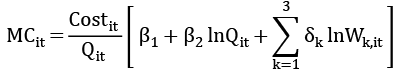
where P is the output price, computed by the ratio of total revenues to total assets, and MS is the marginal cost, obtained by regressing the following translog cost function:

 (4)
(4)
In the translog cost function above, Cost refers to total costs and Q refers to total assets, W1, W2, and W3 represent input prices for labor (expressed as the ratio of personnel costs to total assets), physical capital (quantified as the ratio of other non-interest costs to fixed assets), and funding (indicated by the ratio of interest costs to deposits), respectively. Subsequently, we utilize the coefficients derived from the translog cost function estimation to compute the marginal cost using the following formulation:
 (5)
(5)
3.2 Model Specification
We regress the model of bank opacity that highlights diversification as the primary explanatory variable and control for several key factors as follows:
 (6)
(6)
where Opacity, Diversification, Bank, and Macro are respective measures for bank opacity, diversification, bank-level controls, and macroeconomic control variables. Motivated by the prior literature, in vector Bank we have bank risk, capital equity, bank size, and bank return; in vector Macro we allow for economic cycles and the financial crisis.1 All of these controls are defined in Table 1. vi is the bank-fixed effect, and εi,t is the error term. To avoid reverse causality and take into account the lagged earnings management of banks, we lag our independent variables. As it is standard in the banking literature, the standard errors are clustered at the bank level.
We also take an extra step to shed more light on our findings by exploring how the effects of bank diversification on opacity depend on bank competition. To this end, we extend our baseline model to include an interaction term as follows:

 (7)
(7)
The interaction term between bank diversification and competition, Diversificationi,t–1 × Competitioni,t–1, is the key variable under our regression strategy applied in this extended model. It indicates whether there is any differentiation in the management of bank earnings to business model variations according to bank competition, measured by different proxies of banking market structures.
We advance fixed effects regressions described above (suggested by the Hausman test) using corrected Driscoll-Kraay standard errors that offer estimations robust to cross-sectional and temporal dependence (Hoechle, 2007). As a precautionary measure, we acknowledge a concern that our model specification may suffer from other potential endogeneity issues that could bias our results, such as measurement errors or omitted variables. To address this issue and better encompass the enduring characteristics of earnings opacity, we establish a dynamic model of earnings opacity, incorporating the lagged dependent variable as a regressor.
To conduct dynamic regressions, we use the generalized method of moments (GMM) estimator. The initial form of GMM for dynamic panels, known as difference GMM, involves differencing all regressors and utilizing the lagged levels of the regressors as instruments (Arellano & Bond, 1991). The more advanced form, called system GMM, incorporates both the original equation in levels and its first-differenced version, allowing for the inclusion of additional instruments to significantly improve estimation efficiency (Blundell & Bond, 1998). Consequently, we opt for the system GMM estimator to achieve better results. Specifically, to prevent the excessive increase of instruments in all GMM specifications, we consider the lagged dependent variable as endogenous and treat all independent variables as exogenous (Danisman & Tarazi, 2024; Roodman, 2009). The exogenous variables serve as their own instruments, while for the endogenous variables, we use the second and third lags as instruments. Given our small sample size, we calculate the two-step standard errors using Windmeijer’s (2005) finite-sample correction to ensure reliable GMM estimation results. Besides, while using this estimator, we need some diagnostic tests to confirm its validity.
3.3 Data
We gather annual data of commercial banks in Vietnam through their financial reports. Economic growth data is sourced from the World Development Indicators. To construct efficient diversification measures and avoid noise and spurious associations, we eliminate bank-year observations with negative values of disaggregate components. We also demand each sample bank to publish at least five consecutive years of financial reports to gain robust estimates in the dynamic GMM model. Due to data availability, our sample period runs from 2007 to 2022, with a total of 35 banks and 432 observations. A summary of descriptive statistics for variables employed is provided in Table 1. Overall, these preliminary statistics suggest that the heterogeneity across banks in the sample is large enough to gain reliable estimates.
Table 1
Descriptive Statistics for Variables
|
|
Mean |
SD |
Min |
Max |
Description |
|
IncomeDiver |
0.344 |
0.146 |
0.071 |
0.623 |
Income diversification following the HHI index, calculated by one minus the sum of squared shares of income components |
|
AssetDiver |
0.521 |
0.100 |
0.322 |
0.680 |
Assets diversification following the HHI index, calculated by one minus the sum of squared shares of asset components |
|
FundDiver |
0.503 |
0.124 |
0.218 |
0.714 |
Funding diversification following the HHI index, calculated by one minus the sum of squared shares of funding components |
|
LoanDiver |
0.750 |
0.063 |
0.578 |
0.816 |
Loan portfolio diversification following the HHI index, calculated by one minus the sum of squared shares of sectoral loans |
|
Opacity |
0.007 |
0.005 |
0.001 |
0.023 |
Magnitude of discretionary loan loss provisions |
|
Lerner |
0.443 |
0.078 |
0.279 |
0.591 |
(Out price – Marginal cost)/Output price |
|
MS5 |
0.592 |
0.056 |
0.550 |
0.733 |
Five largest banks’ total assets/The banking system’s total assets |
|
HHImarket |
0.089 |
0.016 |
0.077 |
0.131 |
The sum of squared asset market shares of all banks |
|
NPL |
2.192 |
1.295 |
0.418 |
6.100 |
Non-performing loans/Gross loans (%) |
|
Capital |
10.118 |
4.742 |
4.444 |
23.838 |
Capital equity/Total assets (%) |
|
Size |
32.012 |
1.258 |
29.738 |
34.610 |
Natural logarithm of total assets |
|
ROA |
1.573 |
0.877 |
0.167 |
3.896 |
Return on assets (%) |
|
GDP |
5.902 |
1.432 |
2.600 |
8.000 |
GDP growth rate (%) |
|
Crisis |
0.198 |
0.399 |
0.000 |
1.000 |
Crisis dummy equal to 1 for the years 2007–2009, and 0 otherwise |
4. Empirical Results
4.1 Baseline Regression Results
We start our analysis with the baseline model, where we control bank-level factors only as in Table 2, and then we extend the model by adding macroeconomic controls as in Table 3. Both fixed effects and GMM regressions are employed. The coefficient on income diversification is negative and statistically significant in all columns of Tables 2–3, regardless of the model variant and the regression technique, supporting Hypothesis 1B that income diversification decreases bank opacity. The economic significance of the impact is also acceptable. For example, based on the fully developed model in columns 1 and 5 of Table 3, we infer that a one standard deviation increase in our income diversification proxy (0.146) may lead to a 0.0003–0.0005 (0.0022*0.146–0.0035*0.146) units drop in bank opacity. These variations are reasonable, given that the mean of the opacity variable is 0.007. The finding is at odds with the evidence obtained by Trsn et al. (2019) on US banks that bank earnings management increases with income diversification due to increased information asymmetry. Our result also challenges the finding in Lartey et al. (2022) for the UK banking sector while they look into the relationship in the short term, but lends support for their conclusion about the negative impact of income diversification on earnings opacity in the long term.
Table 2
Opacity Estimations Without Macro Controls
|
|
Dependent variable: Magnitude of discretionary loan loss provisions |
||||||||
|
Fixed effects regressions (columns 1–4) |
|
System GMM regressions (columns 5–8) |
|||||||
|
(1) |
(2) |
(3) |
(4) |
|
(5) |
(6) |
(7) |
(8) |
|
|
Lagged dependent variable |
|
|
|
|
|
0.6395*** |
0.6119*** |
0.5805*** |
0.6257*** |
|
|
|
|
|
|
|
(0.0277) |
(0.0497) |
(0.0550) |
(0.0505) |
|
IncomeDiver |
–0.0039* |
|
|
|
|
–0.0019** |
|
|
|
|
|
(0.0019) |
|
|
|
|
(0.0009) |
|
|
|
|
AssetDiver |
|
–0.0106*** |
|
|
|
|
–0.0046*** |
|
|
|
|
|
(0.0019) |
|
|
|
|
(0.0016) |
|
|
|
FundDiver |
|
|
–0.0086*** |
|
|
|
|
–0.0025* |
|
|
|
|
|
(0.0018) |
|
|
|
|
(0.0013) |
|
|
LoanDiver |
|
|
|
–0.0024 |
|
|
|
|
–0.0096** |
|
|
|
|
|
(0.0091) |
|
|
|
|
(0.0045) |
|
NPL |
–0.0000 |
–0.0001 |
–0.0001 |
–0.0000 |
|
–0.0002* |
–0.0003*** |
–0.0002*** |
–0.0001 |
|
|
(0.0001) |
(0.0001) |
(0.0001) |
(0.0001) |
|
(0.0001) |
(0.0001) |
(0.0001) |
(0.0001) |
|
Capital |
0.0004*** |
0.0003*** |
0.0003*** |
0.0003*** |
|
0.0003*** |
0.0002*** |
0.0002*** |
0.0003*** |
|
|
(0.0001) |
(0.0000) |
(0.0001) |
(0.0001) |
|
(0.0001) |
(0.0001) |
(0.0001) |
(0.0001) |
|
Size |
0.0019*** |
0.0019*** |
0.0016*** |
0.0021*** |
|
0.0013*** |
0.0010*** |
0.0011*** |
0.0013*** |
|
|
(0.0002) |
(0.0002) |
(0.0002) |
(0.0002) |
|
(0.0002) |
(0.0002) |
(0.0002) |
(0.0002) |
|
ROA |
–0.0000 |
–0.0000 |
0.0004 |
0.0002 |
|
–0.0005** |
–0.0004*** |
–0.0002 |
–0.0007*** |
|
|
(0.0003) |
(0.0003) |
(0.0004) |
(0.0003) |
|
(0.0002) |
(0.0001) |
(0.0002) |
(0.0001) |
|
Observations |
397 |
397 |
397 |
397 |
|
397 |
397 |
397 |
397 |
|
Banks |
35 |
35 |
35 |
35 |
|
35 |
35 |
35 |
35 |
|
R-squared |
0.130 |
0.147 |
0.154 |
0.104 |
|
|
|
|
|
|
Instruments |
|
|
|
|
|
26 |
26 |
26 |
26 |
|
AR(1) test |
|
|
|
|
|
0.002 |
0.001 |
0.001 |
0.003 |
|
AR(2) test |
|
|
|
|
|
0.978 |
0.749 |
0.616 |
0.116 |
|
Hansen test |
|
|
|
|
|
0.462 |
0.633 |
0.567 |
0.570 |
|
Note. Standard errors are in parentheses. *** =p<0.01, ** =p<0.05, * p<0.1. |
|||||||||
We now examine how asset diversification affects bank opacity. The coefficient on asset diversification is negative and statistically significant across all related columns in Tables 2–3, implying that greater complexity in asset portfolios may reduce bank earnings management. Quantitatively, the results in columns 2 and 6 in Table 3 suggest that a one standard deviation increase in asset diversification (0.100) is associated with a 0.0006–0.0012 (0.0059*0.100–0.0115*0.100) units decrease in bank opacity. Next, when the diversification variable is in the form of funding, a similar pattern to those reported is observed. Particularly, the coefficient on funding diversification retains its negative sign and statistical significance in columns 3 and 7 of Tables 2 and 3, indicating less earnings opacity in funding-diversified banks. Based on the estimates in fully developed models of Table 3, we realize that a one standard deviation increase in our measure of funding diversification (0.124) may cause a 0.0004–0.0012 (0.0032*0.124–0.0094*0.124) units decrease in earnings opacity.
Table 3
Opacity estimations with macro controls
|
|
Dependent variable: Magnitude of discretionary loan loss provisions |
||||||||
|
Fixed effects regressions (columns 1–4) |
System GMM regressions (columns 5–8) |
||||||||
|
(1) |
(2) |
(3) |
(4) |
(5) |
(6) |
(7) |
(8) |
||
|
Lagged dependent variable |
|
|
|
|
0.5918*** |
0.5304*** |
0.5176*** |
0.5565*** |
|
|
|
|
|
|
|
(0.0261) |
(0.0455) |
(0.0477) |
(0.0479) |
|
|
IncomeDiver |
–0.0035* |
|
|
|
–0.0022*** |
|
|
|
|
|
|
(0.0020) |
|
|
|
(0.0008) |
|
|
|
|
|
AssetDiver |
|
–0.0115*** |
|
|
|
–0.0059*** |
|
|
|
|
|
|
(0.0019) |
|
|
|
(0.0019) |
|
|
|
|
FundDiver |
|
|
–0.0094*** |
|
|
|
–0.0032** |
|
|
|
|
|
|
(0.0015) |
|
|
|
(0.0013) |
|
|
|
LoanDiver |
|
|
|
–0.0024 |
|
|
|
–0.0085** |
|
|
|
|
|
|
(0.0089) |
|
|
|
(0.0044) |
|
|
NPL |
0.0001 |
–0.0002 |
–0.0001 |
–0.0000 |
–0.0001 |
–0.0002** |
–0.0002** |
–0.0001 |
|
|
|
(0.0002) |
(0.0001) |
(0.0001) |
(0.0001) |
(0.0001) |
(0.0001) |
(0.0001) |
(0.0001) |
|
|
Capital |
0.0003*** |
0.0002*** |
0.0002*** |
0.0003*** |
0.0003*** |
0.0002** |
0.0002*** |
0.0002*** |
|
|
|
(0.0001) |
(0.0000) |
(0.0000) |
(0.0000) |
(0.0001) |
(0.0001) |
(0.0001) |
(0.0001) |
|
|
Size |
0.0016*** |
0.0008** |
0.0004*** |
0.0012*** |
0.0012*** |
0.0008*** |
0.0009*** |
0.0011*** |
|
|
|
(0.0005) |
(0.0003) |
(0.0001) |
(0.0003) |
(0.0003) |
(0.0003) |
(0.0002) |
(0.0002) |
|
|
ROA |
0.0002 |
0.0001 |
0.0006 |
0.0003 |
–0.0003* |
–0.0002 |
–0.0000 |
–0.0004*** |
|
|
|
(0.0002) |
(0.0002) |
(0.0004) |
(0.0002) |
(0.0002) |
(0.0001) |
(0.0002) |
(0.0001) |
|
|
GDP |
0.0003 |
–0.0000 |
0.0001 |
0.0003 |
0.0002 |
0.0004* |
0.0006** |
0.0002* |
|
|
|
(0.0002) |
(0.0002) |
(0.0002) |
(0.0002) |
(0.0003) |
(0.0002) |
(0.0002) |
(0.0001) |
|
|
Crisis |
–0.0006 |
–0.0020*** |
–0.0020*** |
–0.0015** |
0.0003 |
–0.0003 |
0.0001 |
–0.0004 |
|
|
|
(0.0007) |
(0.0004) |
(0.0003) |
(0.0006) |
(0.0003) |
(0.0004) |
(0.0004) |
(0.0004) |
|
|
Observations |
397 |
397 |
397 |
397 |
397 |
397 |
397 |
397 |
|
|
Banks |
35 |
35 |
35 |
35 |
35 |
35 |
35 |
35 |
|
|
R-squared |
0.136 |
0.168 |
0.176 |
0.121 |
|
|
|
|
|
|
Instruments |
|
|
|
|
28 |
28 |
28 |
28 |
|
|
AR(1) test |
|
|
|
|
0.002 |
0.001 |
0.001 |
0.003 |
|
|
AR(2) test |
|
|
|
|
0.948 |
0.760 |
0.625 |
0.127 |
|
|
Hansen test |
|
|
|
|
0.446 |
0.496 |
0.412 |
0.599 |
|
|
Note. Standard errors are in parentheses. *** =p<0.01, ** =p<0.05, * p<0.1. |
|||||||||
Finally, in columns 4 and 8 of Tables 2 and 3, the coefficients of loan portfolio diversification are negative and significant in most columns, meaning that diversification in this dimension likely has a negative effect on financial information disclosure. In terms of economic significance, our dynamic models (columns 8 of Tables 2 and 3) show that a one standard deviation increase of loan portfolio diversification (0.063) leads to a 0.0005–0.0006 (0.0085*0.063–0.0096*0.063) units decrease in bank opacity.
Overall, our analysis consistently demonstrates that diversified banks engage in decreased earnings manipulations via discretionary loan loss provisions. This finding completely corroborates Hypothesis 1B. The impact of diversification on opacity is significant not only for the aspect of income diversification, as witnessed with mixed evidence in the existing literature, but also for other diversification dimensions of assets, funding, and loan portfolios. This finding is entirely novel in the literature regarding how bank business models drive earnings manipulations. Collectively, our evidence is in line with the monitoring hypothesis, which claims that diversification is linked with greater complexity and stricter scrutiny from outsiders, thus justifying that earnings manipulation might be discouraged in diversified banks (Acharya et al., 2006; Yu, 2008). Based on this finding, regulators should consider the benefits of diversification when designing oversight mechanisms. Since diversified banks are subjected to stricter scrutiny, regulations should be tailored to ensure that such scrutiny is effective and that it leverages the complexity of diversified operations to prevent earnings manipulation. Besides, policymakers might want to encourage banks to diversify their operations. By providing incentives for diversification, regulators can leverage the natural deterrent against earnings manipulation that comes with increased complexity and external monitoring.
4.2 Augmented Regression Results
We add to the baseline model the variable of bank competition and the interaction term of diversification and competition. Tables 4, 5, and 6 provide our results for the interaction of different diversification measures with the Lerner index, top market shares, and the market concentration index, respectively. Across all tables, we document that diversification is negatively associated with bank opacity, and the associations are significant for all diversification dimensions. This pattern firmly supports the notion that earnings management is less severe for more diversified banks.
Regarding the moderating role of the Lerner index in the diversification and opacity relationship as reported in Table 4, we find that the interaction term is positive and statistically significant in all regressions. Given that the Lerner index refers to the reverse level of bank competition, our overall conclusion for this set of results is that a higher level of competition in the banking system strengthens earnings manipulations at diversified banks. This conclusion holds for all different forms of bank diversification under research.
Table 4
The Interaction of Bank Diversification and Lerner Index
|
|
Dependent variable: Magnitude of discretionary loan loss provisions |
||||||||
|
Fixed effects regressions (columns 1–4) |
|
System GMM regressions (columns 5–8) |
|||||||
|
(1) |
(2) |
(3) |
(4) |
|
(5) |
(6) |
(7) |
(8) |
|
|
Lagged dependent variable |
|
|
|
|
|
0.5807*** |
0.5575*** |
0.5449*** |
0.5006*** |
|
|
|
|
|
|
|
(0.0405) |
(0.0435) |
(0.0460) |
(0.0422) |
|
IncomeDiver |
–0.0244*** |
|
|
|
|
–0.0024*** |
|
|
|
|
|
(0.0034) |
|
|
|
|
(0.0008) |
|
|
|
|
IncomeDiver*Lerner |
0.0553*** |
|
|
|
|
0.0051* |
|
|
|
|
|
(0.0073) |
|
|
|
|
(0.0031) |
|
|
|
|
AssetDiver |
|
–0.0143*** |
|
|
|
|
–0.0094*** |
|
|
|
|
|
(0.0017) |
|
|
|
|
(0.0018) |
|
|
|
AssetDiver*Lerner |
|
0.0124** |
|
|
|
|
0.0185*** |
|
|
|
|
|
(0.0056) |
|
|
|
|
(0.0049) |
|
|
|
FundDiver |
|
|
–0.0121*** |
|
|
|
|
–0.0049*** |
|
|
|
|
|
(0.0017) |
|
|
|
|
(0.0014) |
|
|
FundDiver*Lerner |
|
|
0.0117*** |
|
|
|
|
0.0133*** |
|
|
|
|
|
(0.0030) |
|
|
|
|
(0.0029) |
|
|
LoanDiver |
|
|
|
–0.0180*** |
|
|
|
|
–0.0083*** |
|
|
|
|
|
(0.0047) |
|
|
|
|
(0.0028) |
|
LoanDiver*Lerner |
|
|
|
0.0434*** |
|
|
|
|
0.0333*** |
|
|
|
|
|
(0.0077) |
|
|
|
|
(0.0031) |
|
Bank-level controls |
Yes |
Yes |
Yes |
Yes |
|
Yes |
Yes |
Yes |
Yes |
|
Macro controls |
Yes |
Yes |
Yes |
Yes |
|
Yes |
Yes |
Yes |
Yes |
|
Observations |
397 |
397 |
397 |
397 |
|
397 |
397 |
397 |
397 |
|
Banks |
35 |
35 |
35 |
35 |
|
35 |
35 |
35 |
35 |
|
R-squared |
0.225 |
0.183 |
0.194 |
0.279 |
|
|
|
|
|
|
Instruments |
|
|
|
|
|
30 |
30 |
30 |
30 |
|
AR(1) test |
|
|
|
|
|
0.003 |
0.001 |
0.001 |
0.002 |
|
AR(2) test |
|
|
|
|
|
0.714 |
0.858 |
0.649 |
0.398 |
|
Hansen test |
|
|
|
|
|
0.448 |
0.588 |
0.620 |
0.571 |
|
Note. Standard errors are in parentheses. *** =p<0.01, **= p<0.05, *= p<0.1. |
|||||||||
Turning to the interaction of bank diversification and top market shares, we still find an accentuating role of bank competition. Precisely, as shown in Table 5, the interaction terms between the MS5 variable and each of the diversification measures enter the regressions with positive and statistically significant coefficients in most columns. Equivalently, competition still motivates banks’ information disclosure incentives at diversified banks when we rely on the market concentration index for analysis. Examining the outcomes presented in Table 6, it is noteworthy that the coefficient associated with the interaction term between various forms of diversification and the HHImarket competition proxy is consistently positive and holds statistical significance across all columns.
Table 5
The Interaction of Bank Diversification and Top Market Shares
|
|
Dependent variable: Magnitude of discretionary loan loss provisions |
|||||||
|
Fixed effects regressions (columns 1–4) |
System GMM regressions (columns 5–8) |
|||||||
|
(1) |
(2) |
(3) |
(4) |
(5) |
(6) |
(7) |
(8) |
|
|
Lagged dependent variable |
|
|
|
|
0.5530*** |
0.4815*** |
0.4872*** |
0.4573*** |
|
|
|
|
|
|
(0.0568) |
(0.0481) |
(0.0412) |
(0.0578) |
|
IncomeDiver |
–0.0040* |
|
|
|
–0.0500*** |
|
|
|
|
|
(0.0022) |
|
|
|
(0.0157) |
|
|
|
|
IncomeDiver*MS5 |
0.0024 |
|
|
|
0.0885*** |
|
|
|
|
|
(0.0014) |
|
|
|
(0.0272) |
|
|
|
|
AssetDiver |
|
–0.0465*** |
|
|
|
–0.1012*** |
|
|
|
|
|
(0.0089) |
|
|
|
(0.0220) |
|
|
|
AssetDiver*MS5 |
|
0.0539*** |
|
|
|
0.1653*** |
|
|
|
|
|
(0.0121) |
|
|
|
(0.0384) |
|
|
|
FundDiver |
|
|
–0.0405*** |
|
|
|
–0.0771*** |
|
|
|
|
|
(0.0093) |
|
|
|
(0.0240) |
|
|
FundDiver*MS5 |
|
|
0.0535*** |
|
|
|
0.1319*** |
|
|
|
|
|
(0.0155) |
|
|
|
(0.0423) |
|
|
LoanDiver |
|
|
|
–0.0362** |
|
|
|
–0.0340** |
|
|
|
|
|
(0.0123) |
|
|
|
(0.0148) |
|
LoanDiver*MS5 |
|
|
|
0.0549* |
|
|
|
0.0560** |
|
|
|
|
|
(0.0268) |
|
|
|
(0.0228) |
|
MS5 |
0.0041 |
0.0418*** |
0.0522*** |
–0.0404 |
0.0380* |
0.0972*** |
0.0729** |
–0.0283 |
|
|
(0.0113) |
(0.0095) |
(0.0134) |
(0.0277) |
(0.0198) |
(0.0293) |
(0.0287) |
(0.0262) |
|
Bank-level controls |
Yes |
Yes |
Yes |
Yes |
Yes |
Yes |
Yes |
Yes |
|
Macro controls |
Yes |
Yes |
Yes |
Yes |
Yes |
Yes |
Yes |
Yes |
|
Observations |
397 |
397 |
397 |
397 |
397 |
397 |
397 |
397 |
|
Banks |
35 |
35 |
35 |
35 |
35 |
35 |
35 |
35 |
|
R-squared |
0.157 |
0.213 |
0.308 |
0.285 |
|
|
|
|
|
Instruments |
|
|
|
|
30 |
30 |
30 |
30 |
|
AR(1) test |
|
|
|
|
0.002 |
0.000 |
0.000 |
0.002 |
|
AR(2) test |
|
|
|
|
0.915 |
0.573 |
0.496 |
0.144 |
|
Hansen test |
|
|
|
|
0.538 |
0.567 |
0.529 |
0.384 |
|
Note. Standard errors are in parentheses. ***=p<0.01, ** =p<0.05, *= p<0.1. |
||||||||
In summary, our findings reveal that while bank diversification leads to decreased opacity in bank earnings on average, this impact is conditioned by bank competition, consistent with Hypothesis 2. In more detail, the decrease in bank earnings manipulation caused by diversification of all forms is intensified by the surge of competition in the banking market. Furthermore, the assessments from two structural measures and one non-structural index of bank competition provide identical evidence. Our consistent findings suggest that complex banks confront greater scrutiny from external agents, especially in highly competitive markets (Nickell, 1996), and react by decreasing earnings management. Hence, competition is an essential channel in stimulating the impact of bank diversification on earnings management practices.
Table 6
The Interaction of Bank Diversification and Market Concentration Index
|
|
Dependent variable: Magnitude of discretionary loan loss provisions |
|||||||
|
Fixed effects regressions (columns 1–4) |
System GMM regressions (columns 5–8) |
|||||||
|
(1) |
(2) |
(3) |
(4) |
(5) |
(6) |
(7) |
(8) |
|
|
Lagged dependent variable |
|
|
|
|
0.5490*** |
0.5096*** |
0.5123*** |
0.4698*** |
|
|
|
|
|
|
(0.0549) |
(0.0448) |
(0.0429) |
(0.0530) |
|
IncomeDiver |
–0.0043* |
|
|
|
–0.0220*** |
|
|
|
|
|
(0.0022) |
|
|
|
(0.0085) |
|
|
|
|
IncomeDiver*HHImarket |
0.0222** |
|
|
|
0.2762*** |
|
|
|
|
|
(0.0092) |
|
|
|
(0.1028) |
|
|
|
|
AssetDiver |
|
–0.0301*** |
|
|
|
–0.0430*** |
|
|
|
|
|
(0.0053) |
|
|
|
(0.0064) |
|
|
|
AssetDiver*HHImarket |
|
0.1708*** |
|
|
|
0.4330*** |
|
|
|
|
|
(0.0381) |
|
|
|
(0.0807) |
|
|
|
FundDiver |
|
|
–0.0254*** |
|
|
|
–0.0271*** |
|
|
|
|
|
(0.0048) |
|
|
|
(0.0062) |
|
|
FundDiver*HHImarket |
|
|
0.1790*** |
|
|
|
0.2948*** |
|
|
|
|
|
(0.0472) |
|
|
|
(0.0795) |
|
|
LoanDiver |
|
|
|
–0.0190** |
|
|
|
–0.0180** |
|
|
|
|
|
(0.0067) |
|
|
|
(0.0078) |
|
LoanDiver*HHImarket |
|
|
|
0.1732* |
|
|
|
0.2002*** |
|
|
|
|
|
(0.0894) |
|
|
|
(0.0766) |
|
HHImarket |
0.0367* |
0.1339*** |
0.1670*** |
–0.1252 |
–0.0796 |
0.1843*** |
0.1094** |
–0.0663 |
|
|
(0.0191) |
(0.0196) |
(0.0388) |
(0.0779) |
(0.0589) |
(0.0580) |
(0.0506) |
(0.0693) |
|
Bank-level controls |
Yes |
Yes |
Yes |
Yes |
Yes |
Yes |
Yes |
Yes |
|
Macro controls |
Yes |
Yes |
Yes |
Yes |
Yes |
Yes |
Yes |
Yes |
|
Observations |
397 |
397 |
397 |
397 |
397 |
397 |
397 |
397 |
|
Banks |
35 |
35 |
35 |
35 |
35 |
35 |
35 |
35 |
|
R-squared |
0.158 |
0.212 |
0.312 |
0.276 |
|
|
|
|
|
Instruments |
|
|
|
|
30 |
30 |
30 |
30 |
|
AR(1) test |
|
|
|
|
0.002 |
0.000 |
0.001 |
0.002 |
|
AR(2) test |
|
|
|
|
0.901 |
0.642 |
0.589 |
0.151 |
|
Hansen test |
|
|
|
|
0.548 |
0.439 |
0.458 |
0.376 |
|
Note. Standard errors are in parentheses. *** =p<0.01, ** =p<0.05, * =p<0.1. |
||||||||
4.3 Robustness Checks
In this subsection, we conduct further robustness checks to demonstrate whether these checks still confirm our main findings. First, it is essential to mention that this paper utilizes ordinary least squares to break down the loan loss provisions variable into its predicted and residual parts, with the residuals used as the dependent variable in the second regression. This two-step approach can produce biased coefficients and incorrect standard errors (Chen et al., 2018). Therefore, as a robustness check, we use discretionary loan loss provisions as the dependent variable, incorporating the variables from the first stage (Equation 1) as well as all control variables from the second stage (Equation 7). As shown in Table 7, the results remain unaltered.
Table 7
Robustness Checks with all Control Variables
|
|
Dependent variable: Magnitude of discretionary loan loss provisions |
|||||||
|
(1) |
(2) |
(3) |
(4) |
(5) |
(6) |
(7) |
(8) |
|
|
IncomeDiver |
–0.0081** |
|
|
|
–0.0027** |
|
|
|
|
|
(0.0032) |
|
|
|
(0.0012) |
|
|
|
|
AssetDiver |
|
–0.0190*** |
|
|
|
–0.0063*** |
|
|
|
|
|
(0.0046) |
|
|
|
(0.0023) |
|
|
|
FundDiver |
|
|
–0.0142** |
|
|
|
–0.0091* |
|
|
|
|
|
(0.0065) |
|
|
|
(0.0054) |
|
|
LoanDiver |
|
|
|
–0.0025 |
|
|
|
–0.0062* |
|
|
|
|
|
(0.0062) |
|
|
|
(0.0034) |
|
IncomeDiver*Lerner |
|
|
|
|
0.0079** |
|
|
|
|
|
|
|
|
|
(0.0037) |
|
|
|
|
AssetDiver*Lerner |
|
|
|
|
|
0.0154** |
|
|
|
|
|
|
|
|
|
(0.0064) |
|
|
|
FundDiver*Lerner |
|
|
|
|
|
|
0.0370*** |
|
|
|
|
|
|
|
|
|
(0.0115) |
|
|
LoanDiver*Lerner |
|
|
|
|
|
|
|
0.0304*** |
|
|
|
|
|
|
|
|
|
(0.0042) |
|
Lerner |
|
|
|
|
0.0112*** |
0.0157*** |
0.0260*** |
0.0197*** |
|
|
|
|
|
|
(0.0033) |
(0.0050) |
(0.0057) |
(0.0041) |
|
First-stage controls (Equation 1) |
Yes |
Yes |
Yes |
Yes |
Yes |
Yes |
Yes |
Yes |
|
Second-stage controls (Equation 7) |
Yes |
Yes |
Yes |
Yes |
Yes |
Yes |
Yes |
Yes |
|
Observations |
397 |
397 |
397 |
397 |
397 |
397 |
397 |
397 |
|
Banks |
35 |
31 |
31 |
31 |
31 |
31 |
31 |
31 |
|
R-squared |
0.246 |
0.204 |
0.233 |
0.298 |
0.249 |
0.211 |
0.247 |
0.305 |
|
Note. The table presents the results from the fixed effects model that combines first- and second-stage regressors. Standard errors are in parentheses. *** =p<0.01, ** =p<0.05, * =p<0.1. |
||||||||
Next, we test the sensitivity of our estimates to another choice of bank opacity. To this end, we rely on an alternative version of discretionary loan loss provisions as suggested by Beatty and Liao (2014), which includes the ratio of loan loss allowances to total loans and net charge-offs divided by lagged total loans. We also take the natural logarithm of discretionary loan loss provisions to wipe out the effects of outliers (Tran et al., 2019). We also modify the calculation of bank diversification measures. Following the prior studies, we utilize the ratio of non-interest income to total operating income (NIIShare) as an alternative proxy for income diversification (Meslier et al., 2014; Stiroh & Rumble, 2006), the ratio of non-interest-bearing assets to total assets (NIBAShare) as an alternative proxy for asset diversification (Moudud-Ul-Huq et al., 2018), and the ratio of non-deposit funding to total funding (NDFShare) as an alternative proxy for funding diversification (Fosu et al., 2017). Consistent with Huynh and Dang (2021), we introduce an alternative loan portfolio diversification index computed by the assignment of ten sectoral exposures (LoanDiver10), using the procedure similar to the one applied earlier to the index using six sectoral exposures.2 Likewise, we also change the way we construct our variables of bank competition. As suggested by the literature, we drop the funding price in the translog cost function to calculate an adjusted Lerner index that introduces a “clean” indicator of bank pricing power (Turk Ariss, 2010). We also change the construction of top market shares using an alternative version, obtained by the ratio of the three largest banks’ total assets to the entire banking system’s total assets.
Additionally, we approach another advanced econometric method to replace fixed effects and GMM estimations, given that one could doubt about the efficiency of our results based on a small-size sample. In this regard, we choose the least squares dummy variable corrected (LSDVC) estimator as an alternative technique since it is known as a superior technique that well fits in small and highly unbalanced research samples (Bruno, 2005), which is the situation in our study. It is important to highlight that the LSDVC estimator presumes all explanatory variables, except for the lagged dependent variable, to be strictly exogenous.
We perform regressions based on each alternative design of bank opacity, diversification, competition, or empirical technique while keeping other factors constant. Our main findings are unaffected. To save space, we report the estimates combining all changes in variables and regression methods in this subsection. Our new sets of results for the baseline and extended models of bank opacity are presented in Table 8 and Table 9, respectively. To display the LSDVC results, we select the Anderson and Hsiao version using 50 times of replication (it should be noticed that other LSDVC variants do not affect our conclusions). We find that the coefficients on bank diversification measures and interaction terms remain unaltered. Once again, our estimation results support the negative impact of bank diversification on earnings opacity and the amplifying role of bank competition in this nexus.
Table 8
Robustness Checks for the Baseline Regressions
|
|
Dependent variable: Natural logarithm of discretionary loan loss provisions |
|||
|
|
(1) |
(2) |
(3) |
(4) |
|
Lagged dependent variable |
0.437*** |
0.381*** |
0.360*** |
0.429*** |
|
|
(0.049) |
(0.048) |
(0.036) |
(0.058) |
|
NIIShare |
–0.022*** |
|
|
|
|
|
(0.004) |
|
|
|
|
NIBAShare |
|
–1.933*** |
|
|
|
|
|
(0.567) |
|
|
|
NDFShare |
|
|
–1.104*** |
|
|
|
|
|
(0.223) |
|
|
LoanDiver10 |
|
|
|
–1.056** |
|
|
|
|
|
(0.467) |
|
NPL |
0.090 |
–0.034** |
–0.013 |
0.025 |
|
|
(0.060) |
(0.017) |
(0.019) |
(0.017) |
|
Capital |
–0.005 |
0.019* |
0.025*** |
0.050*** |
|
|
(0.017) |
(0.010) |
(0.009) |
(0.015) |
|
Size |
0.097* |
0.074 |
0.140*** |
0.222*** |
|
|
(0.056) |
(0.051) |
(0.047) |
(0.038) |
|
ROA |
0.206*** |
0.091* |
0.095*** |
–0.044 |
|
|
(0.060) |
(0.054) |
(0.036) |
(0.048) |
|
GDP |
0.041 |
–0.109** |
0.002 |
–0.013 |
|
|
(0.046) |
(0.053) |
(0.050) |
(0.027) |
|
Crisis |
0.211* |
–0.029 |
0.057 |
0.017 |
|
|
(0.121) |
(0.092) |
(0.086) |
(0.091) |
|
Observations |
397 |
397 |
397 |
397 |
|
Banks |
35 |
35 |
35 |
35 |
|
Note. The table presents the LSDVC regression results. Standard errors are in parentheses. ***= p<0.01, **= p<0.05, * =p<0.1. |
||||
Table 9
Robustness Checks for the Augmented Regressions
|
|
Dependent variable: Natural logarithm of discretionary loan loss provisions |
|||||||||||||
|
Competition: Lerner adjusted |
|
Competition: Top three banks |
|
Competition: HHI index market shares |
||||||||||
|
(1) |
(2) |
(3) |
(4) |
|
(5) |
(6) |
(7) |
(8) |
|
(9) |
(10) |
(11) |
(12) |
|
|
Lagged dependent variable |
0.388*** |
0.447*** |
0.264*** |
0.437*** |
|
0.478*** |
0.406*** |
0.435*** |
0.416*** |
|
0.541*** |
0.421*** |
0.444*** |
0.385*** |
|
|
(0.023) |
(0.054) |
(0.052) |
(0.059) |
|
(0.049) |
(0.035) |
(0.033) |
(0.057) |
|
(0.068) |
(0.027) |
(0.023) |
(0.047) |
|
NIIShare |
–0.080*** |
|
|
|
|
–0.144*** |
|
|
|
|
–0.142*** |
|
|
|
|
|
(0.012) |
|
|
|
|
(0.029) |
|
|
|
|
(0.036) |
|
|
|
|
NIIShare* Competition |
0.163*** |
|
|
|
|
0.346*** |
|
|
|
|
1.690*** |
|
|
|
|
|
(0.026) |
|
|
|
|
(0.072) |
|
|
|
|
(0.430) |
|
|
|
|
NIBAShare |
|
–5.795*** |
|
|
|
|
–6.482*** |
|
|
|
|
–5.174*** |
|
|
|
|
|
(1.100) |
|
|
|
|
(0.717) |
|
|
|
|
(0.631) |
|
|
|
NIBAShare* Competition |
|
10.758*** |
|
|
|
|
14.681*** |
|
|
|
|
56.166*** |
|
|
|
|
|
(1.751) |
|
|
|
|
(1.976) |
|
|
|
|
(8.602) |
|
|
|
NDFShare |
|
|
–2.826*** |
|
|
|
|
–9.807*** |
|
|
|
|
–10.684*** |
|
|
|
|
|
(0.496) |
|
|
|
|
(2.162) |
|
|
|
|
(1.199) |
|
|
NDFShare* Competition |
|
|
1.763** |
|
|
|
|
22.849*** |
|
|
|
|
121.564*** |
|
|
|
|
|
(0.754) |
|
|
|
|
(5.506) |
|
|
|
|
(14.419) |
|
|
LoanDiver10 |
|
|
|
–1.587*** |
|
|
|
|
–6.095*** |
|
|
|
|
–0.772* |
|
|
|
|
|
(0.453) |
|
|
|
|
(1.144) |
|
|
|
|
(0.435) |
|
LoanDiver10* Competition |
|
|
|
4.805*** |
|
|
|
|
14.894*** |
|
|
|
|
12.889*** |
|
|
|
|
|
(0.574) |
|
|
|
|
(2.706) |
|
|
|
|
(4.306) |
|
Competition |
3.730*** |
5.398*** |
0.995* |
3.536*** |
|
–2.671 |
–0.659 |
–0.407 |
3.549* |
|
32.038** |
14.242* |
26.876*** |
5.147 |
|
|
(0.537) |
(0.693) |
(0.559) |
(0.362) |
|
(2.616) |
(1.566) |
(2.381) |
(2.021) |
|
(14.215) |
(7.450) |
(7.423) |
(7.813) |
|
Bank-level controls |
Yes |
Yes |
Yes |
Yes |
Yes |
Yes |
Yes |
Yes |
Yes |
Yes |
Yes |
Yes |
||
|
Macro controls |
Yes |
Yes |
Yes |
Yes |
Yes |
Yes |
Yes |
Yes |
Yes |
Yes |
Yes |
Yes |
||
|
Observations |
397 |
397 |
397 |
397 |
|
397 |
397 |
397 |
397 |
|
397 |
397 |
397 |
397 |
|
Banks |
35 |
35 |
35 |
35 |
|
35 |
35 |
35 |
35 |
|
35 |
35 |
35 |
35 |
|
Note. The table presents the LSDVC regression results. Competition measures are displayed at the top of columns. Standard errors are in parentheses. *** =p<0.01, ** =p<0.05, * =p<0.1. |
||||||||||||||
5. Conclusions
This paper examines the effect of bank diversification on earnings opacity in Vietnam from 2007 to 2022. Our estimates consistently indicate the negative link between bank diversification and earnings management. When banks diversify across different dimensions of income, assets, funding, and loan portfolios, it seems that they are less likely to manipulate earnings. In an effort to deepen our finding, we exhibit that the effect of bank diversification on opacity is conditional on bank competition. Specifically, diversified banks should have more substantial incentives to reduce bank opacity when operating in a highly competitive market. Taken together, these findings offer strong support for the monitoring hypothesis.
Our study provides some policy implications, at least from the perspective of emerging markets. Given the downsides that bank opacity creates for outsiders, our findings suggest that a movement toward higher levels of diversification in banking operations could increase the capacity of these outsiders to judge bank quality and outcomes. Vietnam’s monetary authorities have also been actively promoting bank diversification. Policies encouraging banks to expand beyond traditional lending and embrace a broader range of financial services align well with the findings of our study. By diversifying their operations, Vietnamese banks can mitigate risks associated with opacity and provide clearer insights into their financial health and performance, thereby boosting investor confidence and market stability. Alternatively, there is a need to apply complementary measures to enhance market discipline through bank transparency, such as the Basel III regulatory framework, if banks show a highly concentrated business model and consistently stick their operations into conventional banking segments. Besides, our analysis highlights the conditioning role of market competition in the relationship between diversification and opacity. Hence, as banks’ financial information disclosure incentives are more due to the monitoring pressures from external agents, a proper degree of banking competition should be encouraged to boost the favorable influence of diversified business models on bank earnings opacity.
While our study makes valuable contributions, we must acknowledge its limitations. Our research is restricted to focusing on a single market with certain database constraints. Additionally, when aiming to explore moderators and interaction terms to verify the role of bank competition in the relationship between diversification and opacity, it would be beneficial to illustrate marginal effects using plots and confidence intervals. Therefore, we suggest that future research revisit our findings across various countries, employing a more comprehensive approach to gain a deeper understanding of the topic.
References
Abbas,F., & Ali, S. (2022). Dynamics of diversification and banks’ risk-taking and stability: Empirical analysis of commercial banks. Managerial and Decision Economics, 43(4), 1000–1014. https://doi.org/10.1002/MDE.3434
Acharya, V. V., Hasan, I., & Saunders, A. (2006). Should Banks Be Diversified? Evidence from Individual Bank Loan Portfolios. Journal of Business, 79(3), 1355–1412. https://doi.org/10.1086/500679
Allen, F., & Gale, D. (2004). Competition and Financial Stability. Journal of Money, Credit, and Banking, 36(3b), 453–480. https://doi.org/10.1353/mcb.2004.0038
Altamuro, J., & Beatty, A. (2010). How does internal control regulation affect financial reporting? Journal of Accounting and Economics, 49(1–2), 58–74. https://doi.org/10.1016/J.JACCECO.2009.07.002
Arellano, M., & Bond, S. (1991). Some Tests of Specification for Panel Data: Monte Carlo Evidence and an Application to Employment Equations. Review of Economic Studies, 58(2), 277–297. https://doi.org/10.2307/2297968
Barth, M. E., Gomez-Biscarri, J., Kasznik, R., & López-Espinosa, G. (2017). Bank Earnings and Regulatory Capital Management Using Available for Sale Securities. Review of Accounting Studies, 22(4), 1761–1792. https://doi.org/10.1007/S11142-017-9426-Y
Beatty, A., & Liao, S. (2011). Do delays in expected loss recognition affect banks’ willingness to lend? Journal of Accounting and Economics, 52(1), 1–20. https://doi.org/10.1016/J.JACCECO.2011.02.002
Beatty, A., & Liao, S. (2014). Financial accounting in the banking industry: A review of the empirical literature. Journal of Accounting and Economics, 58(2–3), 339–383. https://doi.org/10.1016/J.JACCECO.2014.08.009
Berger, A. N., Klapper, L. F., & Turk-Ariss, R. (2009). Bank Competition and Financial Stability. Journal of Financial Services Research, 35(2), 99–118. https://doi.org/10.1007/s10693-008-0050-7
Blundell, R., & Bond, S. (1998). Initial conditions and moment restrictions in dynamic panel data models. Journal of Econometrics, 87(1), 115–143. https://doi.org/10.1016/S0304-4076(98)00009-8
Boot, A. W. A. (2000). Relationship Banking: What Do We Know? Journal of Financial Intermediation, 9(1), 7–25. https://doi.org/10.1006/jfin.2000.0282
Bruno, G. S. F. (2005). Estimation and Inference in Dynamic Unbalanced Panel-data Models with a Small Number of Individuals. Stata Journal, 5(4), 473–500. https://doi.org/10.1177/1536867x0500500401
Cao, Y. (2022). Bank earnings management and performance reporting of comprehensive income. Journal of Accounting and Public Policy, 41(5). https://doi.org/10.1016/J.JACCPUBPOL.2022.106996
Chen, J., Ezzamel, M., & Cai, Z. (2011). Managerial power theory, tournament theory, and executive pay in China. Journal of Corporate Finance, 17(4), 1176–1199. https://doi.org/10.1016/J.JCORPFIN.2011.04.008
Chen, W. E. I., Hribar, P., & Melessa, S. (2018). Incorrect Inferences When Using Residuals as Dependent Variables. Journal of Accounting Research, 56(3), 751–796. https://doi.org/10.1111/1475-679X.12195
Dang, V. D. (2020). Do non-traditional banking activities reduce bank liquidity creation? Evidence from Vietnam. Research in International Business and Finance, 54. https://doi.org/10.1016/j.ribaf.2020.101257
Dang, V. D., & Huynh, J. (2022). Bank funding, market power, and the bank liquidity creation channel of monetary policy. Research in International Business and Finance, 59. https://doi.org/10.1016/J.RIBAF.2021.101531
Dang, V. D., & Huynh, J. (2023). Bank opacity and stability in an emerging market. International Journal of Emerging Markets. DOI:10.1108/IJOEM-03-2022-0514
Danisman, G. O., & Tarazi, A. (2024). ESG activity and bank lending during financial crises. Journal of Financial Stability, 70, 101206. https://doi.org/10.1016/j.jfs.2023.101206
Datta, S., Iskandar-Datta, M., & Sharma, V. (2011). Product market pricing power, industry concentration and analysts’ earnings forecasts. Journal of Banking and Finance, 35(6), 1352–1366. https://doi.org/10.1016/j.jbankfin.2010.10.016
Dell’Ariccia, G., & Marquez, R. (2006). Lending Booms and Lending Standards. The Journal of Finance, 61(5), 2511–2546. https://doi.org/10.1111/j.1540-6261.2006.01065.x
Desalegn, T. A., & Zhu, H. (2021). Does economic policy uncertainty affect bank earnings opacity? Evidence from China. Journal of Policy Modeling, 43(5), 1000–1015. https://doi.org/10.1016/j.jpolmod.2021.03.006
Flannery, M. J., Kwan, S. H., & Nimalendran, M. (2013). The 2007-2009 financial crisis and bank opaqueness. Journal of Financial Intermediation, 22(1), 55–84. https://doi.org/10.1016/j.jfi.2012.08.001
Fosu, S., Danso, A., Agyei-Boapeah, H., Ntim, C. G., & Murinde, V. (2018). How does banking market power affect bank opacity? Evidence from analysts’ forecasts. International Review of Financial Analysis, 60, 38–52. https://doi.org/10.1016/j.irfa.2018.08.015
Fosu, S., Ntim, C. G., Coffie, W., & Murinde, V. (2017). Bank opacity and risk-taking: Evidence from analysts’ forecasts. Journal of Financial Stability, 33, 81–95. https://doi.org/10.1016/j.jfs.2017.10.009
Hoechle, D. (2007). Robust Standard Errors for Panel Regressions with Cross-Sectional Dependence. Stata Journal, 7(3), 281–312. https://doi.org/10.1177/1536867x070070031
Huang, R., & Ratnovski, L. (2011). The dark side of bank wholesale funding. Journal of Financial Intermediation, 20(2), 248–263. https://doi.org/10.1016/j.jfi.2010.06.003
Huynh, J., & Dang, V. D. (2021). Loan portfolio diversification and bank returns: Do business models and market power matter? Cogent Economics and Finance, 9(1). https://doi.org/10.1080/23322039.2021.1891709
Jensen, M. (1986). Agency Costs of Free Cash Flow, Corporate Finance, and Takeovers. American Economic Review, 76, 323–329.
Jiang, L., Levine, R., & Lin, C. (2016). Competition and Bank Opacity. The Review of Financial Studies, 29(7), 1911–1942. https://doi.org/10.1093/RFS/HHW016
Jin, J. Y., Kanagaretnam, K., & Liu, Y. (2018). Banks’ funding structure and earnings quality. International Review of Financial Analysis, 59, 163–178. https://doi.org/10.1016/j.irfa.2018.08.009
Jones, J. S., Lee, W. Y., & Yeager, T. J. (2013). Valuation and systemic risk consequences of bank opacity. Journal of Banking and Finance, 37(3), 693–706. https://doi.org/10.1016/j.jbankfin.2012.10.028
Jungherr, J. (2018). Bank opacity and financial crises. Journal of Banking and Finance, 97, 157–176. https://doi.org/10.1016/j.jbankfin.2018.09.022
Khan, H. H., Ahmed, R. B., & Gee, C. S. (2016). Bank competition and monetary policy transmission through the bank lending channel: Evidence from ASEAN. International Review of Economics and Finance, 44, 19–39. https://doi.org/10.1016/j.iref.2016.03.003
Kozubovska, M. (2017). The effect of US bank holding companies’ exposure to asset-backed commercial paper conduits on the information opacity and systemic risk. Research in International Business and Finance, 39, 530–545. https://doi.org/10.1016/j.ribaf.2016.09.013
Laeven, L., & Levine, R. (2007). Is there a diversification discount in financial conglomerates? Journal of Financial Economics, 85(2), 331–367. https://doi.org/10.1016/j.jfineco.2005.06.001
Lartey, T., James, G. A., Danso, A., & Boateng, A. (2022). Bank business models, failure risk and earnings opacity: A short- versus long-term perspective. International Review of Financial Analysis, 80. https://doi.org/10.1016/J.IRFA.2022.102041
Maghyereh, A. I., & Yamani, E. (2022). Does bank income diversification affect systemic risk: New evidence from dual banking systems. Finance Research Letters, 47. https://doi.org/10.1016/J.FRL.2022.102814
Meslier, C., Tacneng, R., & Tarazi, A. (2014). Is bank income diversification beneficial? Evidence from an emerging economy. Journal of International Financial Markets, Institutions and Money, 31(1), 97–126. https://doi.org/10.1016/j.intfin.2014.03.007
Morgan, D. P. (2002). Rating Banks: Risk and Uncertainty in an Opaque Industry. American Economic Review, 92(4), 874–888. https://doi.org/10.1257/00028280260344506
Moudud-Ul-Huq, S., Ashraf, B. N., Gupta, A. Das, & Zheng, C. (2018). Does bank diversification heterogeneously affect performance and risk-taking in ASEAN emerging economies? Research in International Business and Finance, 46, 342–362. https://doi.org/10.1016/J.RIBAF.2018.04.007
Najam, H., Abbas, J., Álvarez-Otero, S., Dogan, E., & Sial, M. S. (2022). Towards green recovery: Can banks achieve financial sustainability through income diversification in ASEAN countries? Economic Analysis and Policy, 76, 522–533. https://doi.org/10.1016/J.EAP.2022.09.004
Nguyen, Q. K. (2023). Women in top executive positions, external audit quality and financial reporting quality: Evidence from Vietnam. Journal of Accounting in Emerging Economies. DOI:10.1108/JAEE-03-2023-0059
Nguyen, T. L. A. (2018). Diversification and bank efficiency in six ASEAN countries. Global Finance Journal, 37, 57–78. https://doi.org/10.1016/j.gfj.2018.04.004
Nickell, S. J. (1996). Competition and Corporate Performance. Journal of Political Economy, 104(4), 724–746. https://doi.org/10.1086/262040
Ozili, P. K. (2022). Banking Sector Earnings Management Using Loan Loss Provisions in the Fintech Era. International Journal of Managerial Finance, 18(1), 75–93. https://doi.org/10.1108/IJMF-07-2020-0369
Roodman, D. (2009). How to do xtabond2: An Introduction to Difference and System GMM in Stata. Stata Journal, 9(1), 86–136. https://doi.org/10.1177/1536867X0900900106
Rodríguez-Pérez, G., & van Hemmen, S. (2010). Debt, diversification and earnings management. Journal of Accounting and Public Policy, 29(2), 138–159. https://doi.org/10.1016/J.JACCPUBPOL.2009.10.005
Stiroh, K. J., & Rumble, A. (2006). The dark side of diversification: The case of US financial holding companies. Journal of Banking and Finance, 30(8), 2131–2161. https://doi.org/10.1016/j.jbankfin.2005.04.030
Thomas, S. (2002). Firm diversification and asymmetric information: Evidence from analysts’ forecasts and earnings announcements. Journal of Financial Economics, 64(3), 373–396. https://doi.org/10.1016/S0304-405X(02)00129-0
Tran, D. V., & Ashraf, B. N. (2018). Dividend policy and bank opacity. International Journal of Finance and Economics, 23(2), 186–204. https://doi.org/10.1002/ijfe.1611
Tran, D. V., Hassan, M. K., & Houston, R. (2019). Activity strategies, information asymmetry, and bank opacity. Economic Modelling, 83, 160–172. https://doi.org/10.1016/j.econmod.2019.02.008
Tran, D. V., Hassan, M. K., Houston, R., & Rabbani, M. R. (2022). The impact of bank opacity on bank risk-taking behavior. Journal of Corporate Accounting & Finance, 33(3), 88–101. https://doi.org/10.1002/JCAF.22551
Turk Ariss, R. (2010). On the implications of market power in banking: Evidence from developing countries. Journal of Banking and Finance, 34(4), 765–775. https://doi.org/10.1016/j.jbankfin.2009.09.004
Windmeijer, F. (2005). A finite sample correction for the variance of linear efficient two-step GMM estimators. Journal of Econometrics, 126(1), 25–51. https://doi.org/10.1016/j.jeconom.2004.02.005
Yu, F. (Frank). (2008). Analyst coverage and earnings management. Journal of Financial Economics, 88(2), 245–271. https://doi.org/10.1016/J.JFINECO.2007.05.008
1 We choose not to incorporate a dummy variable for the COVID-19 health crisis of 2020–2021 in our analysis since we observe a high correlation between this variable and GDP, potentially introducing multicollinearity concerns. Further, we believe that the shocks caused by the COVID-19 pandemic could be reflected in economic growth.
2 Interestingly, we also follow the spirit of Laeven and Levine (2007) to generate income-, asset-, and funding-based diversity measures, and we choose another alternative loan portfolio diversification index based on the assignment of eight sectoral exposures. Regardless of any empirical change, our results remain unchanged.